# load packages
library(countdown)
library(tidyverse)
library(gganimate)

# set theme for ggplot2
ggplot2::theme_set(ggplot2::theme_minimal(base_size = 14))

# set width of code output
options(width = 65)

# set figure parameters for knitr
knitr::opts_chunk$set(
  fig.width = 7, # 7" width
  fig.asp = 0.618, # the golden ratio
  fig.retina = 3, # dpi multiplier for displaying HTML output on retina
  fig.align = "center", # center align figures
  dpi = 300 # higher dpi, sharper image
)Interactive reporting + visualization with Shiny I
Lecture 24
Dr. Mine Çetinkaya-Rundel
Duke University
STA 313 - Spring 2023
Warm up
Announcements
- Peer evals due Friday at 5pm
- Meet with your mentor / TAs
- Guest lecture on Tuesday: Allison Horst, ObservableHQ
Setup
From last time
The racing bar chart
Making of the racing bar chart
freedom <- read_csv(here::here("slides/24", "data/freedom.csv"), na = "-")

countries_to_plot <- freedom %>%
  rowwise() %>%
  mutate(sd = sd(c_across(contains("cl_")), na.rm = TRUE)) %>%
  ungroup() %>%
  arrange(desc(sd)) %>%
  relocate(country, sd) %>%
  slice_head(n = 15) %>%
  pull(country)

freedom_to_plot <- freedom %>%
  filter(country %in% countries_to_plot) %>%
  drop_na()

freedom_ranked <- freedom_to_plot %>%
  select(country, contains("cl_")) %>%
  pivot_longer(
    cols = -country,
    names_to = "year",
    values_to = "civil_liberty",
    names_prefix = "cl_",
    names_transform = list(year = as.numeric)
  ) %>%
  group_by(year) %>%
  mutate(rank_in_year = rank(civil_liberty, ties.method = "first")) %>%
  ungroup() %>%
  mutate(is_turkey = if_else(country == "Turkey", TRUE, FALSE))

freedom_faceted_plot <- freedom_ranked %>%
  ggplot(aes(x = civil_liberty, y = factor(rank_in_year))) +
  geom_col(aes(fill = is_turkey), show.legend = FALSE) +
  scale_fill_manual(values = c("gray", "red")) +
  facet_wrap(~year) +
  scale_x_continuous(
    limits = c(-5, 7),
    breaks = 1:7
  ) +
  geom_text(
    hjust = "right",
    aes(label = country),
    x = -1
  ) +
  theme(
    panel.grid.major.y = element_blank(),
    panel.grid.minor.y = element_blank(),
    panel.grid.minor.x = element_blank(),
    axis.text.y = element_blank()
  ) +
  labs(x = NULL, y = NULL)

freedom_bar_race <- freedom_faceted_plot +
  facet_null() +
  geom_text(
    x = 5, y = 1,
    hjust = "left",
    aes(label = as.character(year)),
    size = 10
  ) +
  aes(group = country) +
  transition_time(as.integer(year)) +
  labs(
    title = "Civil liberties rating, {frame_time}",
    subtitle = "1: Highest degree of freedom - 7: Lowest degree of freedom"
  )

animate(
  freedom_bar_race,
  fps      = 2,
  nframes  = 30,
  width    = 900,
  height   = 560,
  renderer = gifski_renderer()
  )
anim_save("gifs/freedom_bar_race.gif")
Shiny: High level view
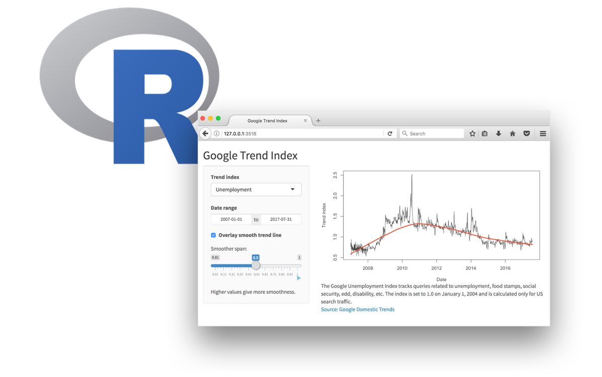
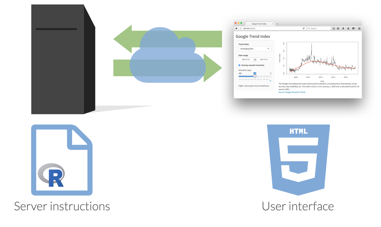
Shiny
Every Shiny app has a webpage that the user visits,
and behind this webpage there is a computer that serves this webpage by running R.
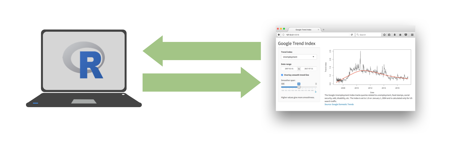
Shiny
When running your app locally, the computer serving your app is your computer.
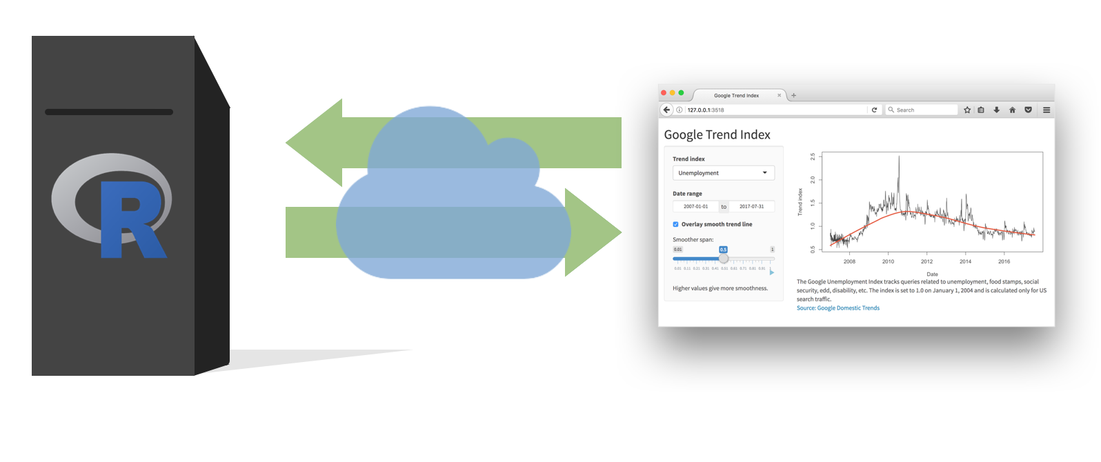
Shiny
When your app is deployed, the computer serving your app is a web server.
Shiny
Demo
- Clone the
ae-21repo. - Navigate to the
goog-indexfolder, and launch the app by opening theapp.Rfile and clicking on Run App. - Close the app by clicking the stop icon
- Select view mode in the drop down menu next to Run App
Anatomy of a Shiny app
What’s in an app?
Data: Ask a manager
Source: Ask a Manager Survey via TidyTuesday
This data does not reflect the general population; it reflects Ask a Manager readers who self-selected to respond, which is a very different group (as you can see just from the demographic breakdown below, which is very white and very female).
Some findings here.
Data: manager
# A tibble: 26,232 × 18
   timestamp          how_old_are_you industry          job_title
   <chr>              <chr>           <chr>             <chr>
 1 4/27/2021 11:02:10 25-34           Education (Highe… Research…
 2 4/27/2021 11:02:22 25-34           Computing or Tech Change &…
 3 4/27/2021 11:02:38 25-34           Accounting, Bank… Marketin…
 4 4/27/2021 11:02:41 25-34           Nonprofits        Program …
 5 4/27/2021 11:02:42 25-34           Accounting, Bank… Accounti…
 6 4/27/2021 11:02:46 25-34           Education (Highe… Scholarl…
 7 4/27/2021 11:02:51 25-34           Publishing        Publishi…
 8 4/27/2021 11:03:00 25-34           Education (Prima… Librarian
 9 4/27/2021 11:03:01 45-54           Computing or Tech Systems …
10 4/27/2021 11:03:02 35-44           Accounting, Bank… Senior A…
# ℹ 26,222 more rows
# ℹ 14 more variables: additional_context_on_job_title <chr>,
#   annual_salary <dbl>, other_monetary_comp <dbl>,
#   currency <chr>, currency_other <chr>,
#   additional_context_on_income <chr>, country <chr>,
#   state <chr>, city <chr>,
#   overall_years_of_professional_experience <chr>, …
Ultimate goal
Interactive reporting with Shiny
Livecoding
Go to the ae-21 project and code along in manager-survey/app-1.R.
Highlights:
- Data pre-processing
- Basic reactivity