# load packages
library(countdown)
library(tidyverse)
library(sf)
library(stars)
library(tmap)
library(gt)
library(scales)
library(colorspace)
library(ggthemes)

# set theme for ggplot2
ggplot2::theme_set(ggplot2::theme_minimal(base_size = 14))

# set width of code output
options(width = 65)

# set figure parameters for knitr
knitr::opts_chunk$set(
  fig.width = 7, # 7" width
  fig.asp = 0.618, # the golden ratio
  fig.retina = 3, # dpi multiplier for displaying HTML output on retina
  fig.align = "center", # center align figures
  dpi = 300 # higher dpi, sharper image
)Tables
Lecture 22
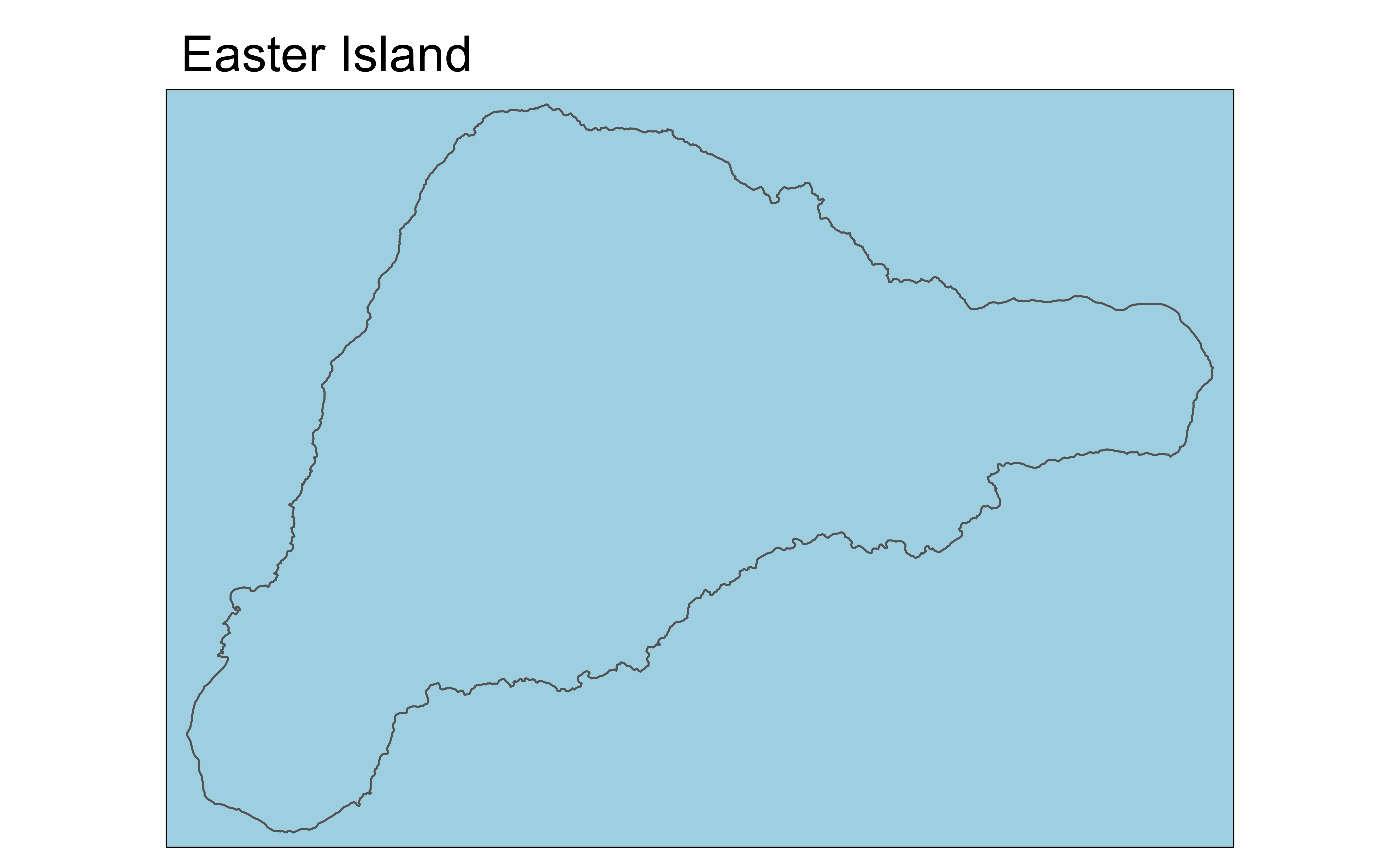
Border
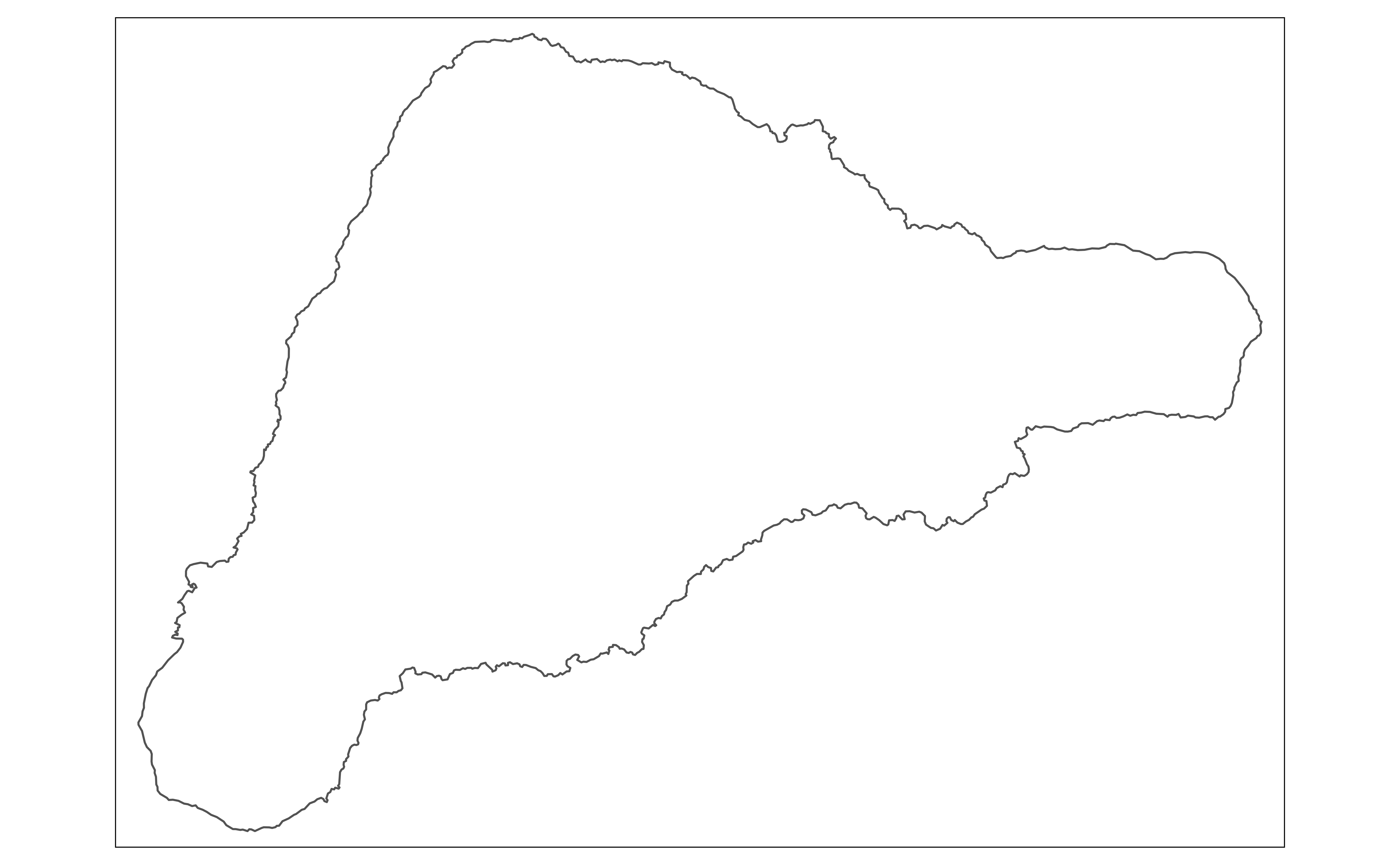
Border + more
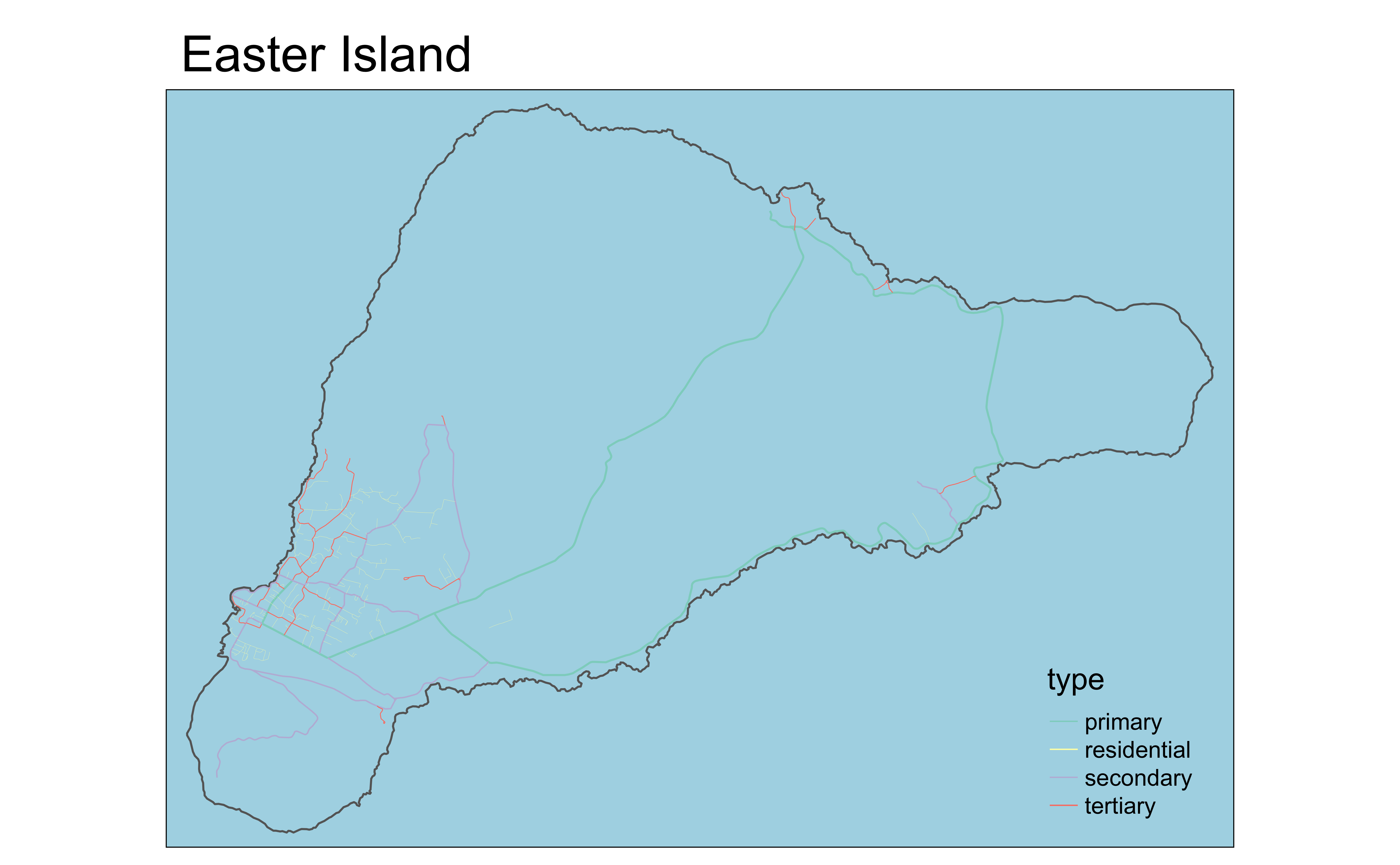
Roads
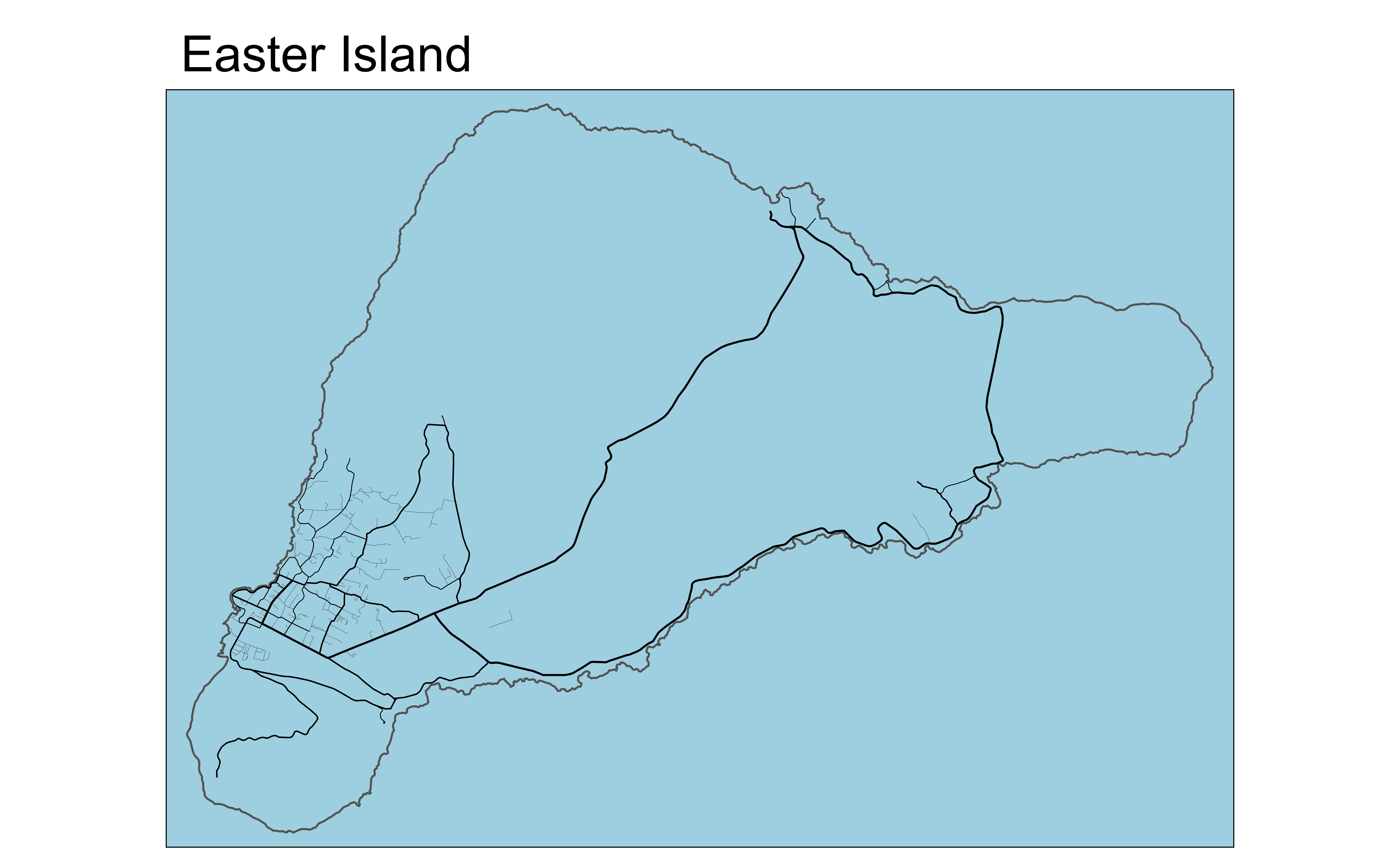
Roads + more
Elevation
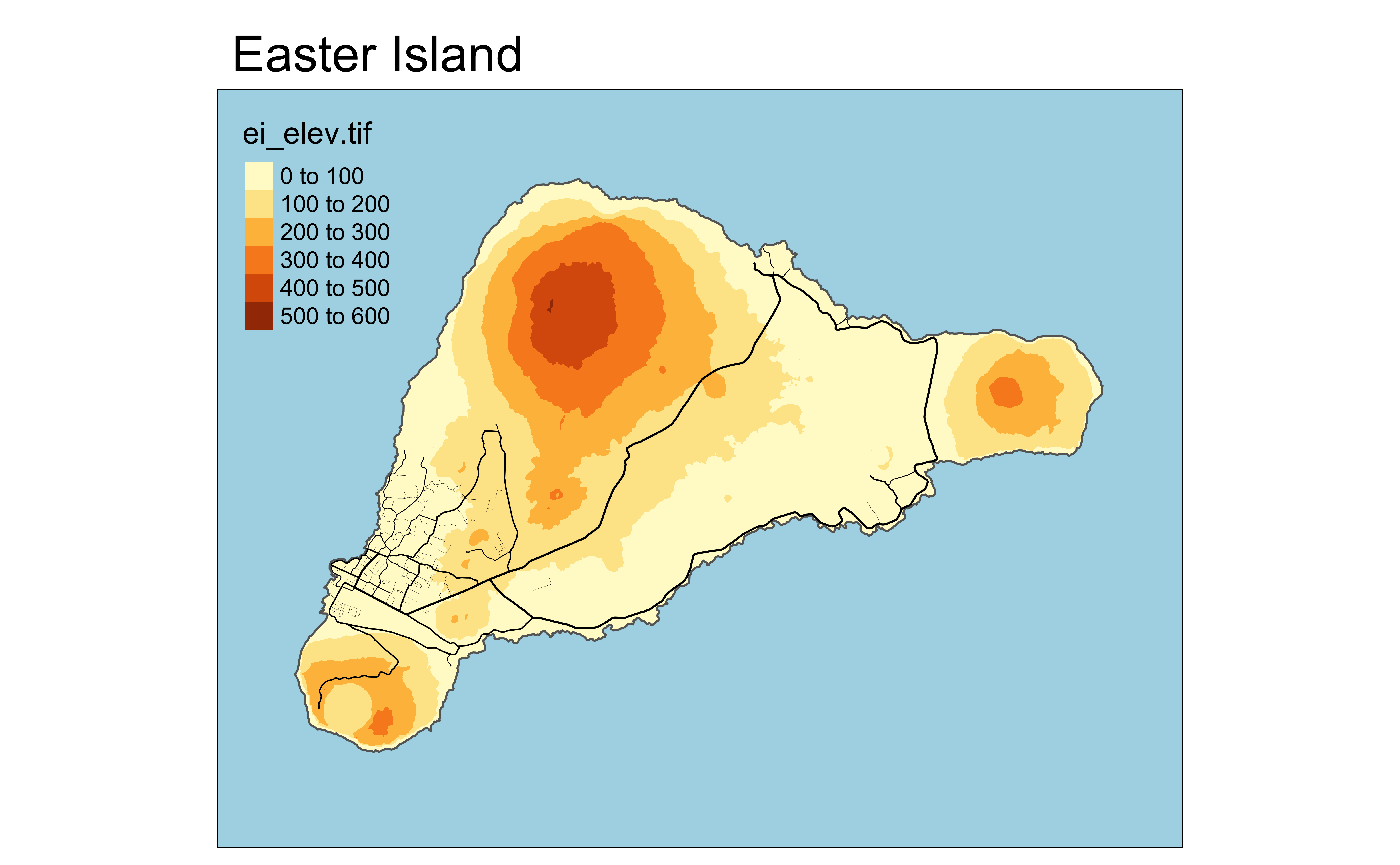
Elevation + more
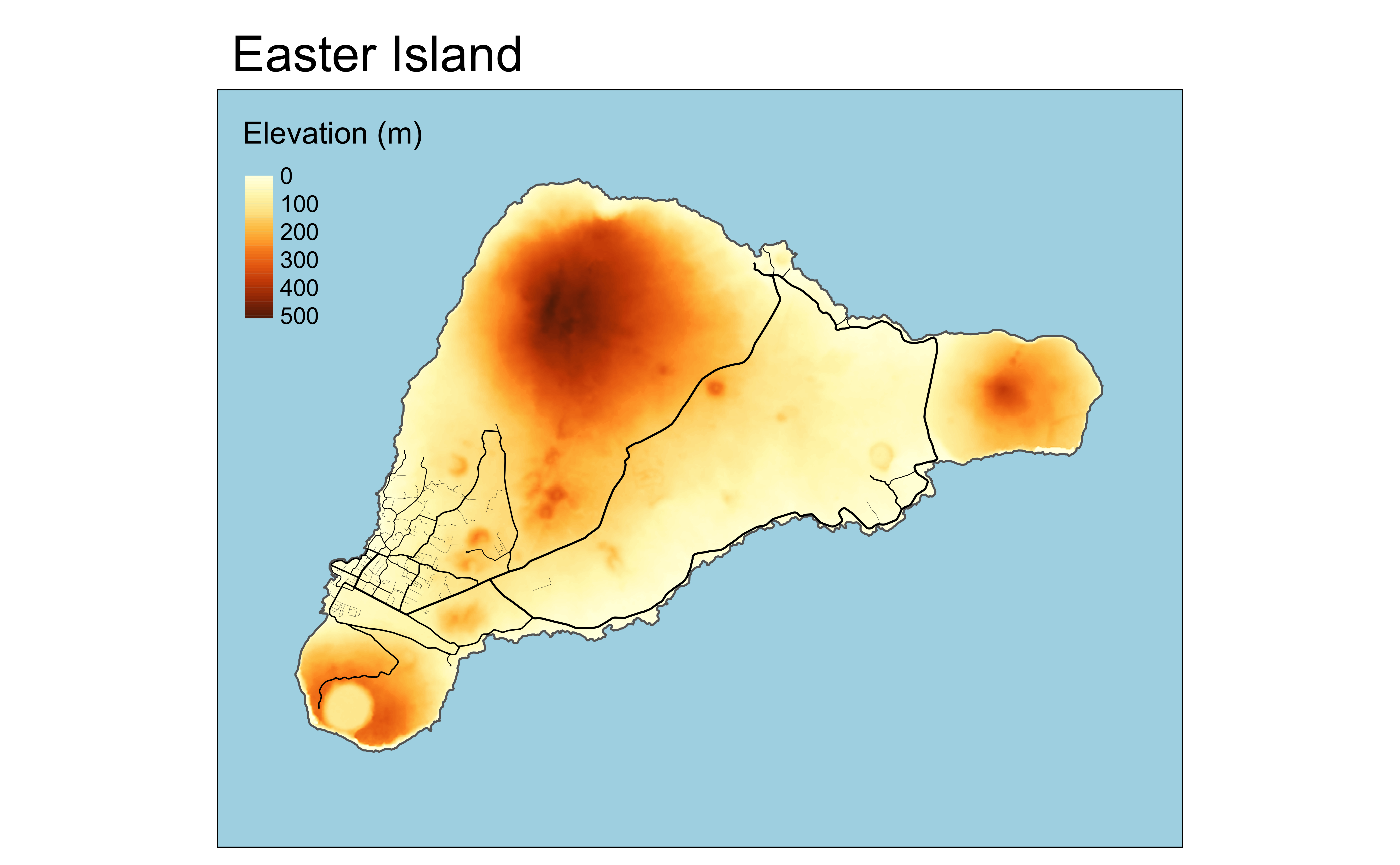
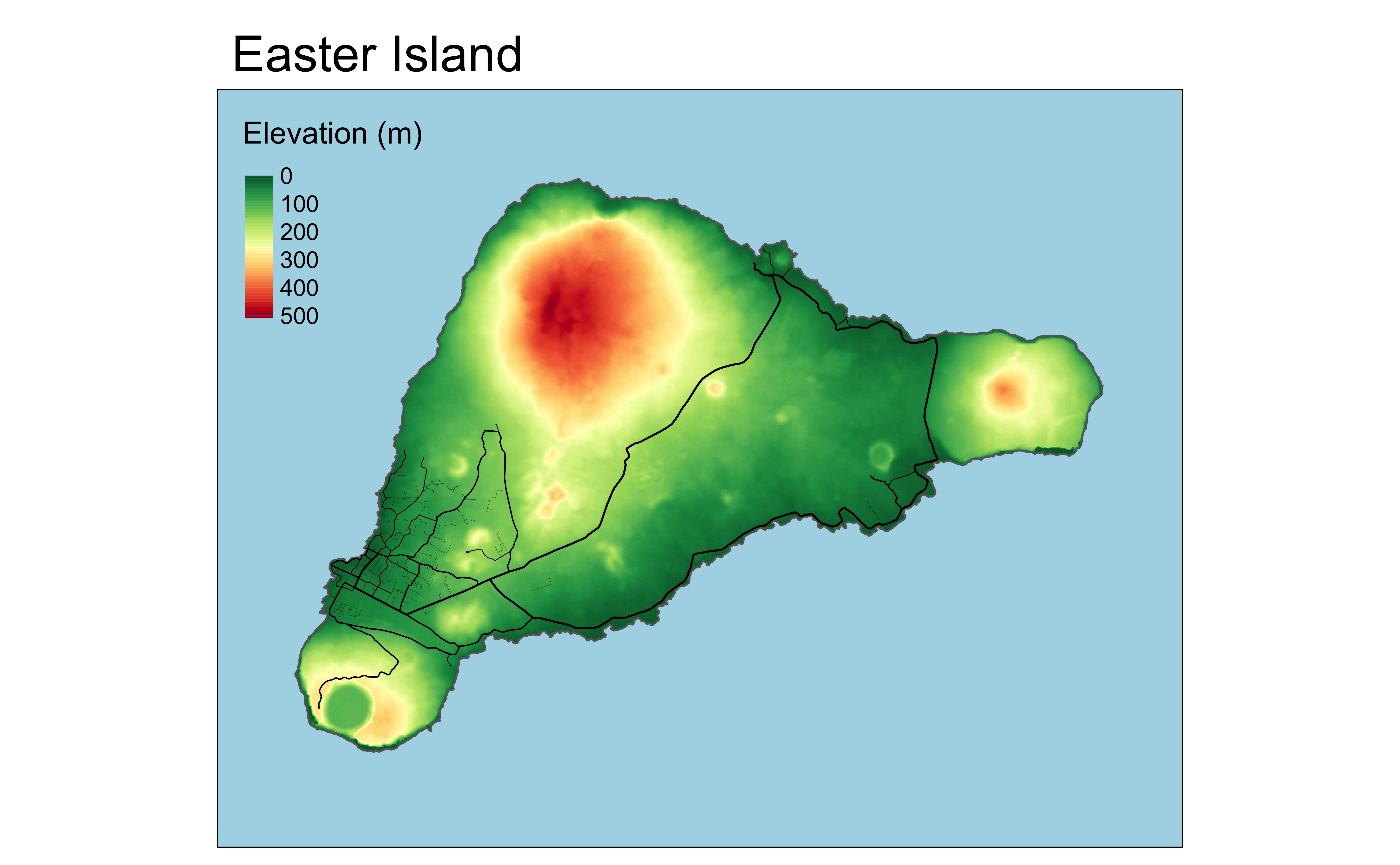
Elevation + even more
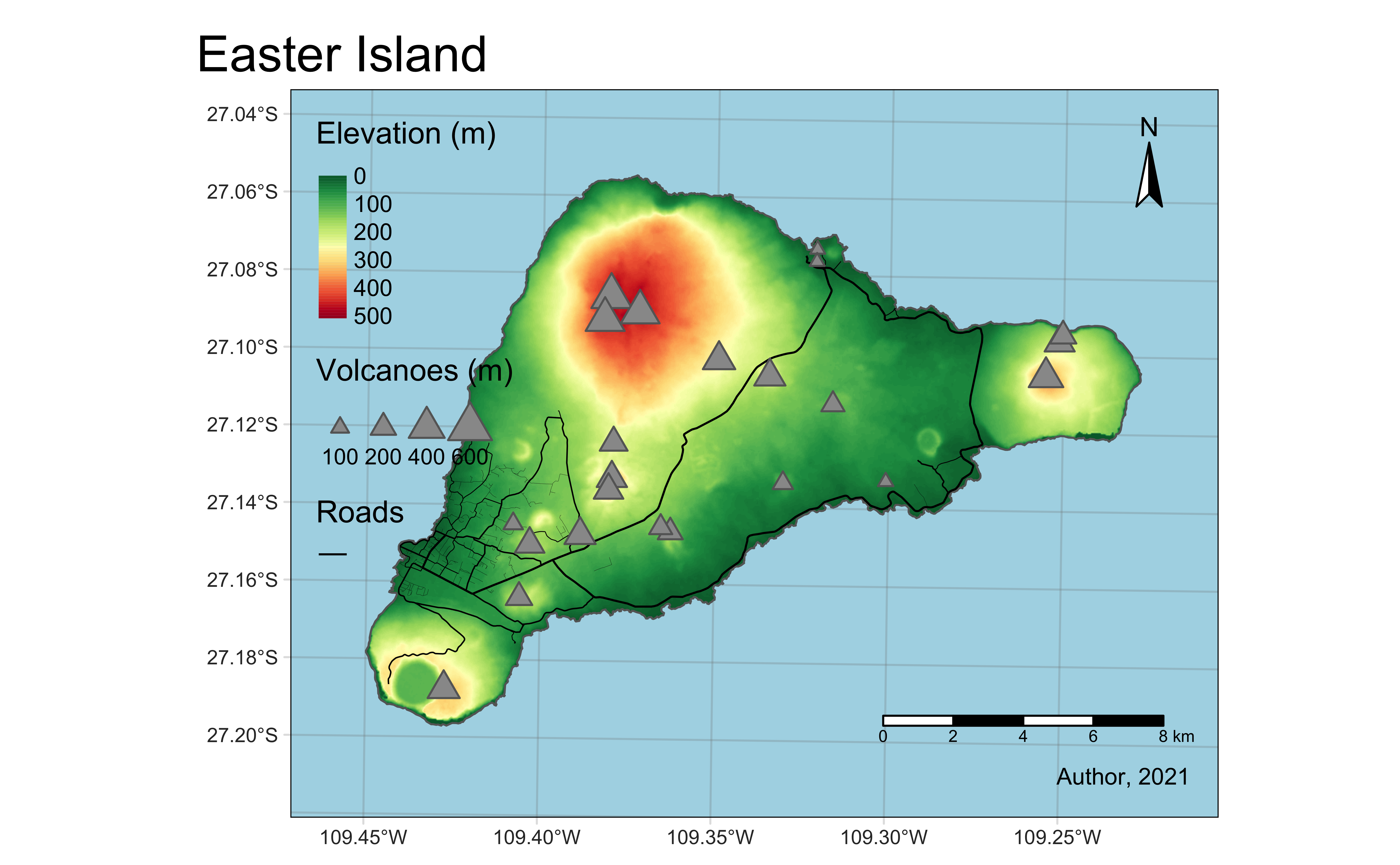
Volcanoes
tm_shape(elev) +
tm_raster(
style = "cont",
title = "Elevation (m)",
palette = "-RdYlGn"
) +
tm_shape(border) +
tm_borders() +
tm_shape(roads) +
tm_lines(
lwd = "strokelwd",
legend.lwd.show = FALSE
) +
tm_shape(
points |> filter(type == "volcano")
) +
tm_symbols(
shape = 24,
size = "elevation",
title.size = "Volcanoes (m)"
) +
tm_layout(
main.title = "Easter Island",
bg.color = "lightblue"
)
Other stuff

plot
# A tibble: 33 × 2
   field                                                     perc
   <chr>                                                    <dbl>
 1 Agriculture and natural resources                      1.91e-2
 2 Architecture and related services                      4.80e-3
 3 Area, ethnic, cultural, gender, and group studies      4.11e-3
 4 Biological and biomedical sciences                     5.80e-2
 5 Business                                               1.92e-1
 6 Communication, journalism, and related programs        4.78e-2
 7 Communications technologies                            2.71e-3
 8 Computer and information sciences                      3.14e-2
 9 Education                                              4.84e-2
10 Engineering                                            5.16e-2
11 Engineering technologies                               9.10e-3
12 English language and literature/letters                2.42e-2
13 Family and consumer sciences/human sciences            1.30e-2
14 Foreign languages, literatures, and linguistics        1.03e-2
15 Health professions and related programs                1.14e-1
16 Homeland security, law enforcement, and firefighting   3.31e-2
17 Legal professions and studies                          2.33e-3
18 Liberal arts and sciences, general studies, and human… 2.30e-2
19 Library science                                        5.22e-5
20 Mathematics and statistics                             1.15e-2
21 Military technologies and applied sciences             1.46e-4
22 Multi/interdisciplinary studies                        2.51e-2
23 Parks, recreation, leisure, and fitness studies        2.59e-2
24 Philosophy and religious studies                       5.84e-3
25 Physical sciences and science technologies             1.59e-2
26 Precision production                                   2.53e-5
27 Psychology                                             6.20e-2
28 Public administration and social services              1.81e-2
29 Social sciences and history                            8.81e-2
30 Theology and religious vocations                       5.12e-3
31 Transportation and materials moving                    2.49e-3
32 Visual and performing arts                             5.06e-2
33 Not classified by field of study 0 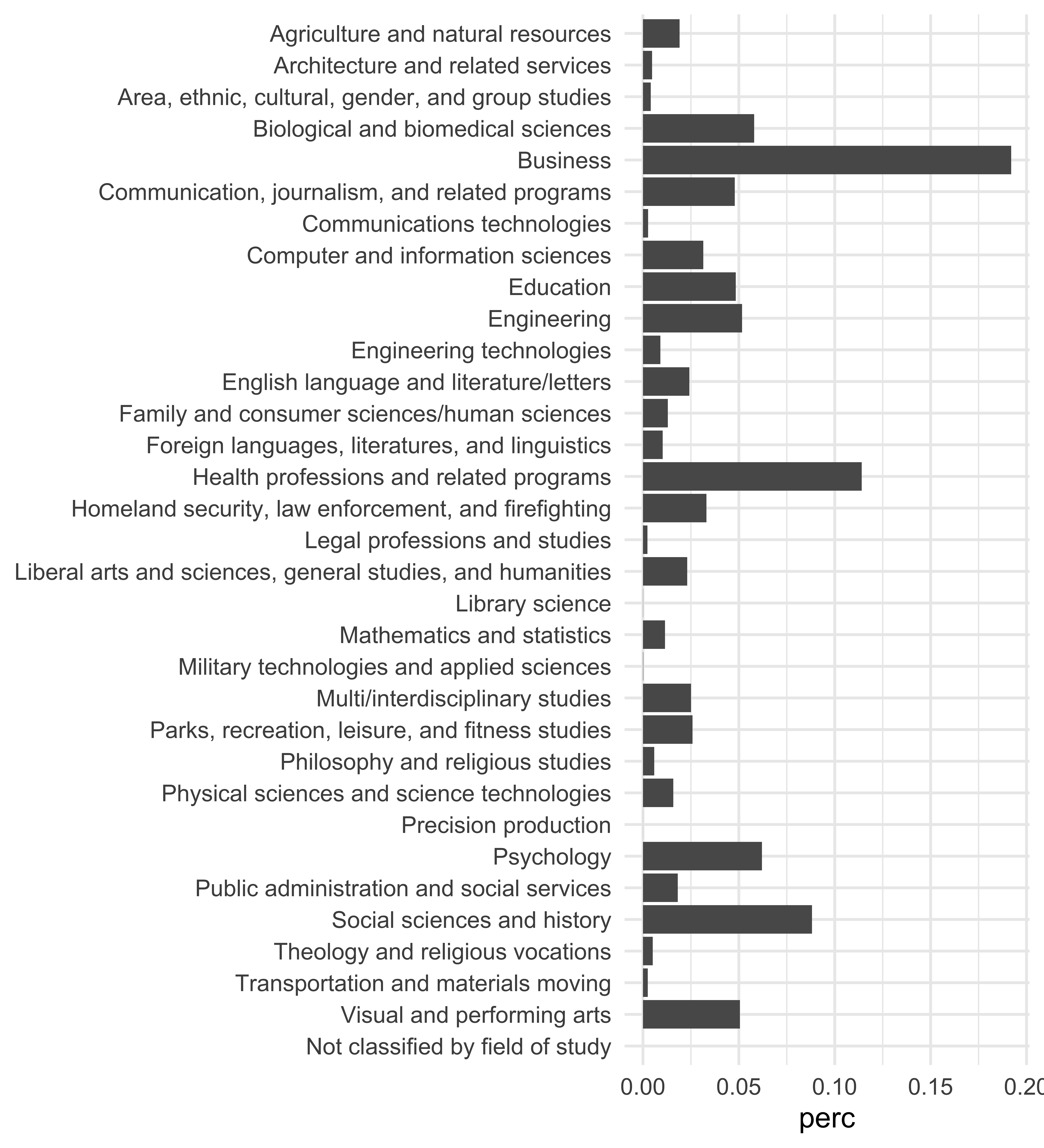
# A tibble: 33 × 2
   field                                                     perc
   <chr>                                                    <dbl>
 1 Business                                               1.92e-1
 2 Health professions and related programs                1.14e-1
 3 Social sciences and history                            8.81e-2
 4 Psychology                                             6.20e-2
 5 Biological and biomedical sciences                     5.80e-2
 6 Engineering                                            5.16e-2
 7 Visual and performing arts                             5.06e-2
 8 Education                                              4.84e-2
 9 Communication, journalism, and related programs        4.78e-2
10 Homeland security, law enforcement, and firefighting   3.31e-2
11 Computer and information sciences                      3.14e-2
12 Parks, recreation, leisure, and fitness studies        2.59e-2
13 Multi/interdisciplinary studies                        2.51e-2
14 English language and literature/letters                2.42e-2
15 Liberal arts and sciences, general studies, and human… 2.30e-2
16 Agriculture and natural resources                      1.91e-2
17 Public administration and social services              1.81e-2
18 Physical sciences and science technologies             1.59e-2
19 Family and consumer sciences/human sciences            1.30e-2
20 Mathematics and statistics                             1.15e-2
21 Foreign languages, literatures, and linguistics        1.03e-2
22 Engineering technologies                               9.10e-3
23 Philosophy and religious studies                       5.84e-3
24 Theology and religious vocations                       5.12e-3
25 Architecture and related services                      4.80e-3
26 Area, ethnic, cultural, gender, and group studies      4.11e-3
27 Communications technologies                            2.71e-3
28 Transportation and materials moving                    2.49e-3
29 Legal professions and studies                          2.33e-3
30 Military technologies and applied sciences             1.46e-4
31 Library science                                        5.22e-5
32 Precision production                                   2.53e-5
33 Not classified by field of study 0 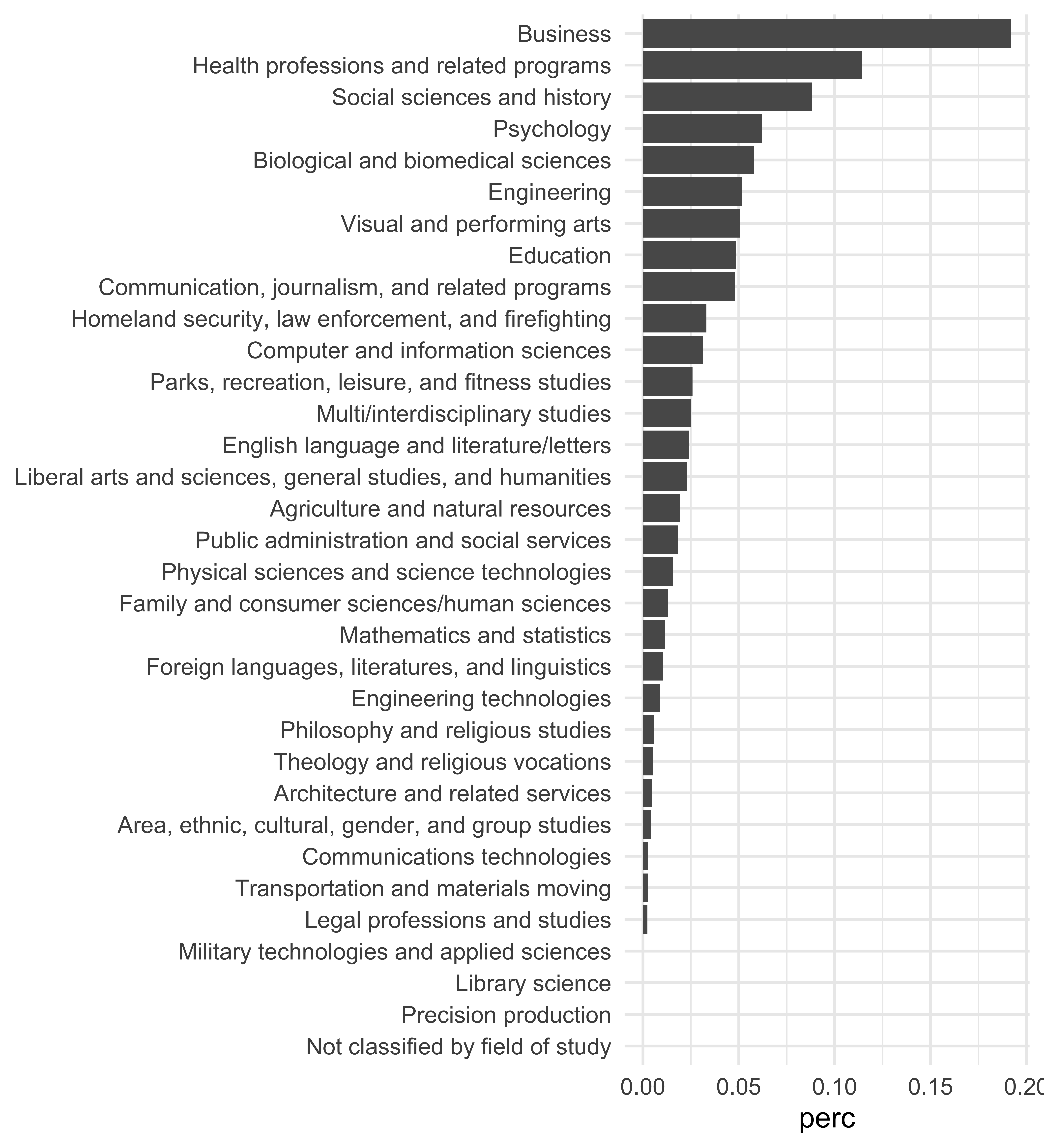
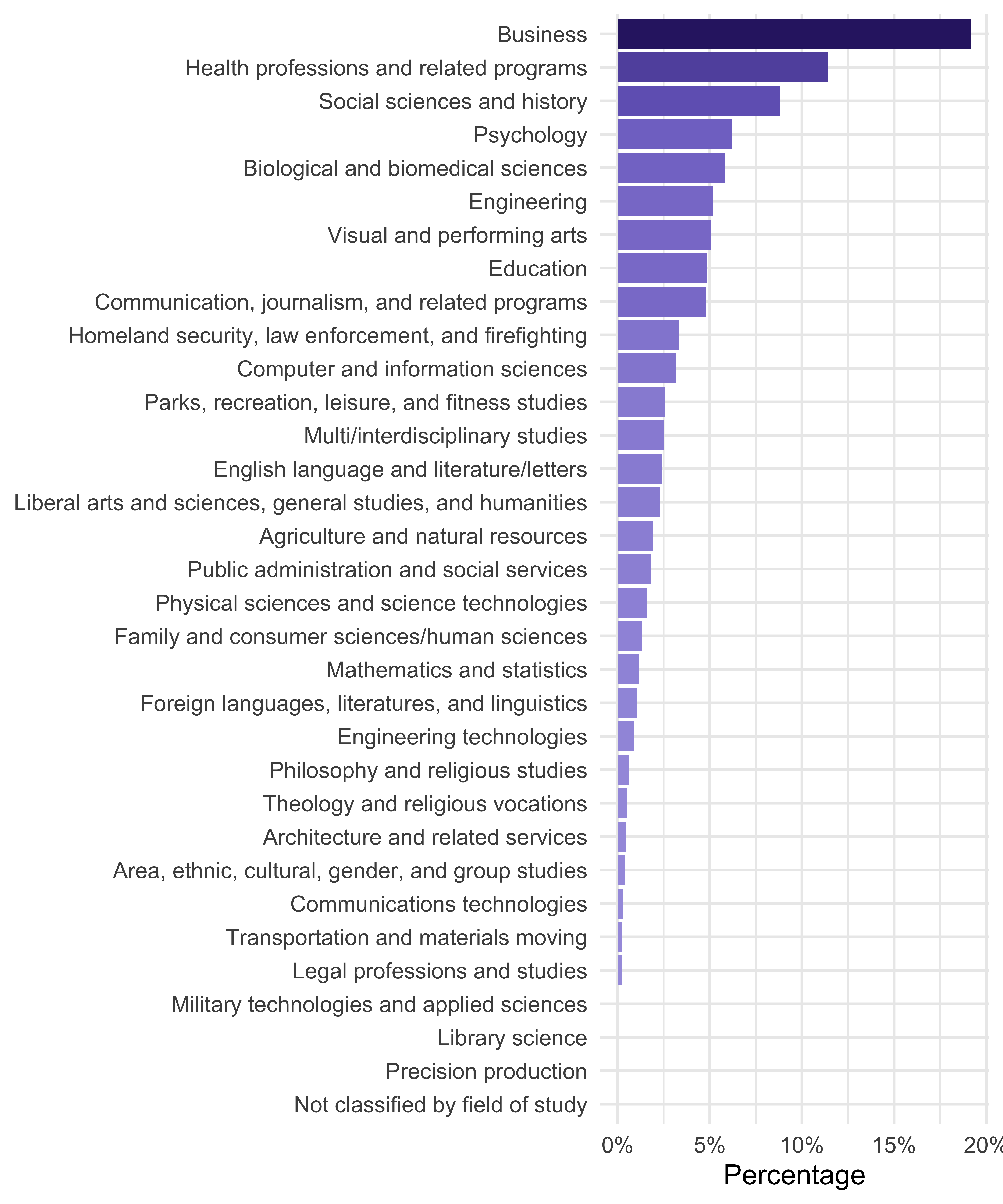
| Field | Percentage |
|---|---|
| Business | 19.2% |
| Health professions and related programs | 11.4% |
| Social sciences and history | 8.8% |
| Psychology | 6.2% |
| Biological and biomedical sciences | 5.8% |
| Engineering | 5.2% |
| Visual and performing arts | 5.1% |
| Education | 4.8% |
| Communication, journalism, and related programs | 4.8% |
| Homeland security, law enforcement, and firefighting | 3.3% |
| Computer and information sciences | 3.1% |
| Parks, recreation, leisure, and fitness studies | 2.6% |
| Multi/interdisciplinary studies | 2.5% |
| English language and literature/letters | 2.4% |
| Liberal arts and sciences, general studies, and humanities | 2.3% |
| Agriculture and natural resources | 1.9% |
| Public administration and social services | 1.8% |
| Physical sciences and science technologies | 1.6% |
| Family and consumer sciences/human sciences | 1.3% |
| Mathematics and statistics | 1.2% |
| Foreign languages, literatures, and linguistics | 1.0% |
| Engineering technologies | 0.9% |
| Philosophy and religious studies | 0.6% |
| Theology and religious vocations | 0.5% |
| Architecture and related services | 0.5% |
| Area, ethnic, cultural, gender, and group studies | 0.4% |
| Communications technologies | 0.3% |
| Transportation and materials moving | 0.2% |
| Legal professions and studies | 0.2% |
| Military technologies and applied sciences | 0.0% |
| Library science | 0.0% |
| Precision production | 0.0% |
| Not classified by field of study | 0.0% |
Or in a plot?
Tables with gt
We will use the gt (Grammar of Tables) package to create tables in R.
The gt philosophy: we can construct a wide variety of useful tables with a cohesive set of table parts.
Source: gt.rstudio.com
Should these data be displayed in a table or a plot?
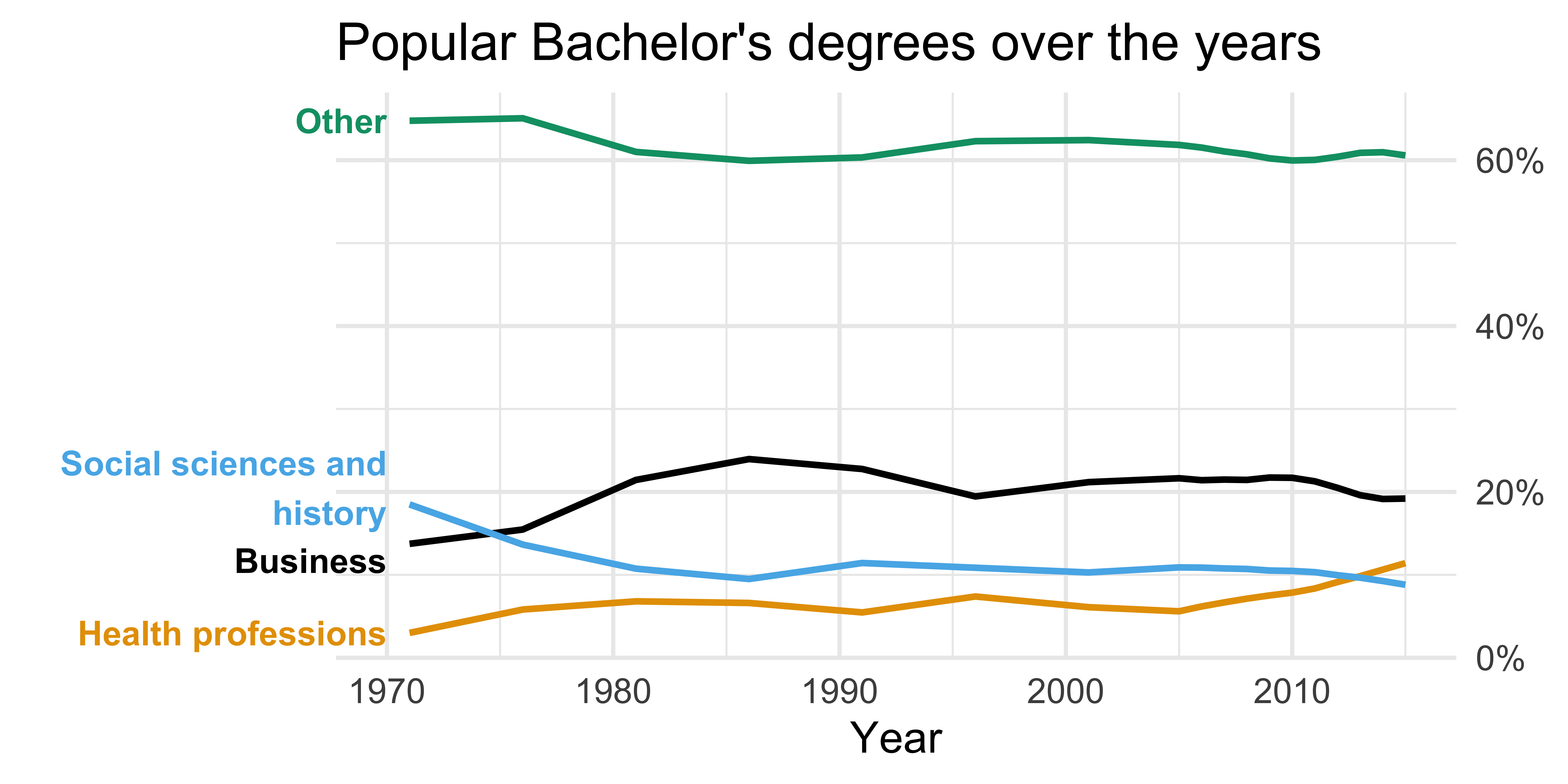
| Popular Bachelor's degrees over the years | ||||||||||||||||||
|---|---|---|---|---|---|---|---|---|---|---|---|---|---|---|---|---|---|---|
| Field | 1971 | 1976 | 1981 | 1986 | 1991 | 1996 | 2001 | 2005 | 2006 | 2007 | 2008 | 2009 | 2010 | 2011 | 2012 | 2013 | 2014 | 2015 |
| Business | 14% | 15% | 21% | 24% | 23% | 19% | 21% | 22% | 21% | 21% | 21% | 22% | 22% | 21% | 20% | 20% | 19% | 19% |
| Health professions | 3% | 6% | 7% | 7% | 5% | 7% | 6% | 6% | 6% | 7% | 7% | 8% | 8% | 8% | 9% | 10% | 11% | 11% |
| Social sciences and history | 18% | 14% | 11% | 9% | 11% | 11% | 10% | 11% | 11% | 11% | 11% | 11% | 10% | 10% | 10% | 10% | 9% | 9% |
| Other | 65% | 65% | 61% | 60% | 60% | 62% | 62% | 62% | 62% | 61% | 61% | 60% | 60% | 60% | 60% | 61% | 61% | 61% |

Add visualizations to your table
Example: Add sparklines to display trend alongside raw data
| Popular Bachelor's degrees over the years | |||||||||||||||||||
|---|---|---|---|---|---|---|---|---|---|---|---|---|---|---|---|---|---|---|---|
| Field | Trend | 1971 | 1976 | 1981 | 1986 | 1991 | 1996 | 2001 | 2005 | 2006 | 2007 | 2008 | 2009 | 2010 | 2011 | 2012 | 2013 | 2014 | 2015 |
| Business |  |
14% | 15% | 21% | 24% | 23% | 19% | 21% | 22% | 21% | 21% | 21% | 22% | 22% | 21% | 20% | 20% | 19% | 19% |
| Health professions |  |
3% | 6% | 7% | 7% | 5% | 7% | 6% | 6% | 6% | 7% | 7% | 8% | 8% | 8% | 9% | 10% | 11% | 11% |
| Social sciences and history |  |
18% | 14% | 11% | 9% | 11% | 11% | 10% | 11% | 11% | 11% | 11% | 11% | 10% | 10% | 10% | 10% | 9% | 9% |
| Other |  |
65% | 65% | 61% | 60% | 60% | 62% | 62% | 62% | 62% | 61% | 61% | 60% | 60% | 60% | 60% | 61% | 61% | 61% |
Livecoding: Recreate this table of popular Bachelor’s degrees awarded over time.
| Popular Bachelor's degrees over the years | |||||||||||||||||||
|---|---|---|---|---|---|---|---|---|---|---|---|---|---|---|---|---|---|---|---|
| Field | Trend | 1971 | 1976 | 1981 | 1986 | 1991 | 1996 | 2001 | 2005 | 2006 | 2007 | 2008 | 2009 | 2010 | 2011 | 2012 | 2013 | 2014 | 2015 |
| Business |  |
14% | 15% | 21% | 24% | 23% | 19% | 21% | 22% | 21% | 21% | 21% | 22% | 22% | 21% | 20% | 20% | 19% | 19% |
| Health professions |  |
3% | 6% | 7% | 7% | 5% | 7% | 6% | 6% | 6% | 7% | 7% | 8% | 8% | 8% | 9% | 10% | 11% | 11% |
| Social sciences and history |  |
18% | 14% | 11% | 9% | 11% | 11% | 10% | 11% | 11% | 11% | 11% | 11% | 10% | 10% | 10% | 10% | 9% | 9% |
| Other |  |
65% | 65% | 61% | 60% | 60% | 62% | 62% | 62% | 62% | 61% | 61% | 60% | 60% | 60% | 60% | 61% | 61% | 61% |
Your turn: Add color to the previous table.
| Popular Bachelor's degrees over the years | |||||||||||||||||||
|---|---|---|---|---|---|---|---|---|---|---|---|---|---|---|---|---|---|---|---|
| Field | Trend | 1971 | 1976 | 1981 | 1986 | 1991 | 1996 | 2001 | 2005 | 2006 | 2007 | 2008 | 2009 | 2010 | 2011 | 2012 | 2013 | 2014 | 2015 |
| Business | |
14% | 15% | 21% | 24% | 23% | 19% | 21% | 22% | 21% | 21% | 21% | 22% | 22% | 21% | 20% | 20% | 19% | 19% |
| Health professions | |
3% | 6% | 7% | 7% | 5% | 7% | 6% | 6% | 6% | 7% | 7% | 8% | 8% | 8% | 9% | 10% | 11% | 11% |
| Social sciences and history | |
18% | 14% | 11% | 9% | 11% | 11% | 10% | 11% | 11% | 11% | 11% | 11% | 10% | 10% | 10% | 10% | 9% | 9% |
| Other | |
65% | 65% | 61% | 60% | 60% | 62% | 62% | 62% | 62% | 61% | 61% | 60% | 60% | 60% | 60% | 61% | 61% | 61% |
10:00
Table inspiration
Storytelling with data: storytellingwithdata.com/blog/2020/9/1/swdchallenge-build-a-table - #23SWDchallenge on Twitter
2022 Posit table contest: Winners of the 2022 Table Contest
- Look out for 2023 table contest anouncement!
![]()