Visualizing geospatial data III

Lecture 20

Dr. Mine Çetinkaya-Rundel

Duke University
STA 313 - Spring 2023

Warm up

Announcements

  • Project proposals for my review due Friday at 5pm
  • HW 5 to be posted soon, HW 4 feedback available

Setup

# load packages
library(countdown)
library(tidyverse)
library(ggnewscale)
library(magick)
library(sf)
library(stars)
library(tmap)

# set theme for ggplot2
ggplot2::theme_set(ggplot2::theme_minimal(base_size = 14))

# set width of code output
options(width = 65)

# set figure parameters for knitr
knitr::opts_chunk$set(
  fig.width = 7, # 7" width
  fig.asp = 0.618, # the golden ratio
  fig.retina = 3, # dpi multiplier for displaying HTML output on retina
  fig.align = "center", # center align figures
  dpi = 300 # higher dpi, sharper image
)

Layering maps

From last time

nc <- read_sf("data/nc_counties/", quiet = TRUE)
air <- read_sf("data/airports/", quiet = TRUE)
hwy <- read_sf("data/us_interstates/", quiet = TRUE)

From last time…

ae-17: Recreate the following visualization.

From last time…

nc_bounds <- st_bbox(nc)

ggplot() +
  geom_sf(data = nc, fill = "gainsboro") +
  geom_sf(data = hwy, color = "#308446", linewidth = 0.75) +
  geom_sf(data = air) +
  ggrepel::geom_label_repel(
    data = air,
    aes(label = IATA, geometry = geometry),
    stat = "sf_coordinates",
    min.segment.length = 0
  ) +
  lims(
    x = c(nc_bounds$xmin, nc_bounds$xmax),
    y = c(nc_bounds$ymin, nc_bounds$ymax)
  ) +
  labs(x = "Longitude", y = "Latitude")

Which counties have airports?

ae-17: On the map of NC you made previously, highlight the counties that have airports.

10:00

Using stars

Spatiotemporal arrays with stars

The stars package provides infrastructure for data cubes, array data with labeled dimensions, with emphasis on arrays where some of the dimensions relate to time and/or space.

Three-dimensional cube:

Multi-dimensional hypercube:

Easter Island

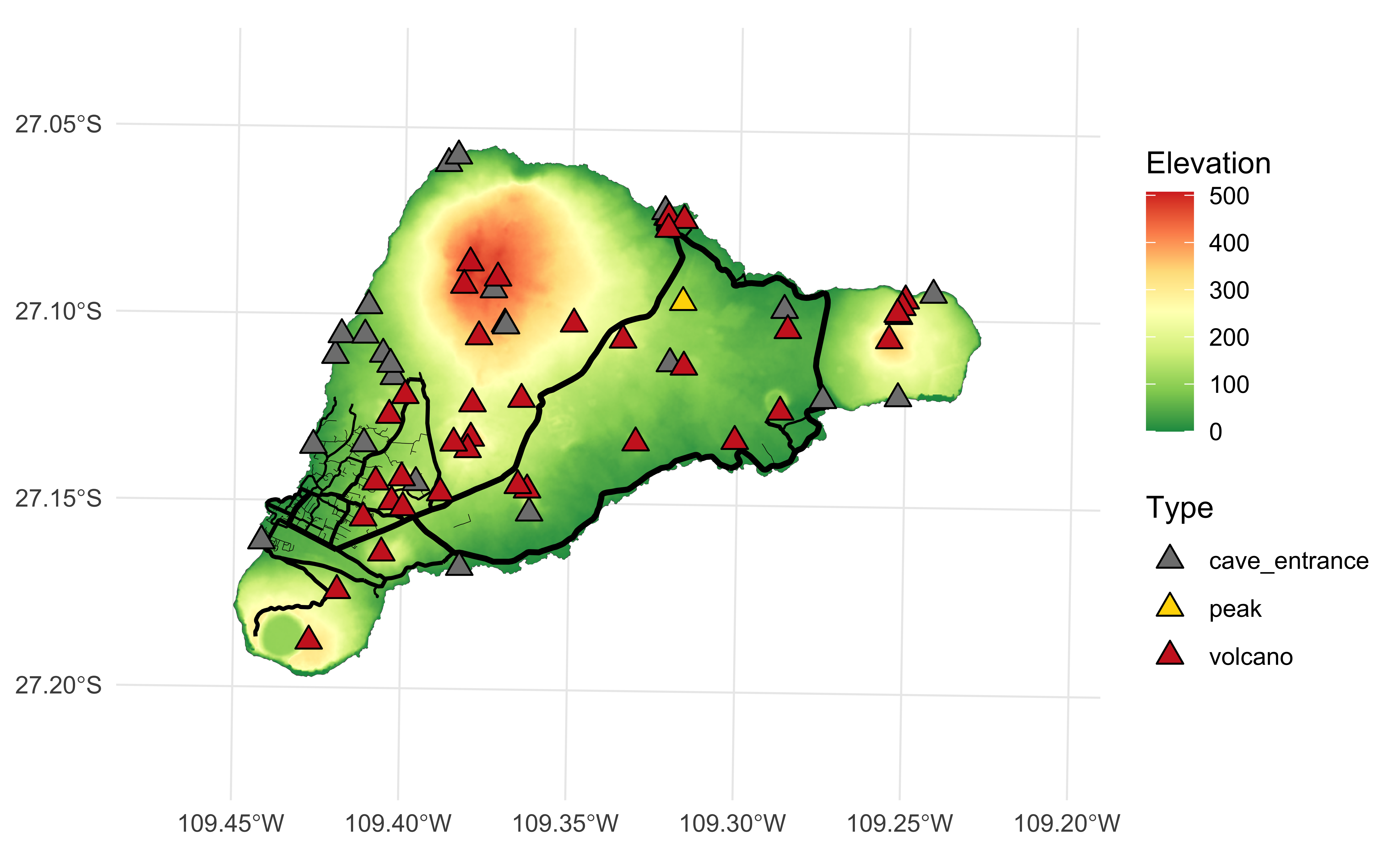
Easter Island (Rapa Nui / Isla de Pascua), a Chilean territory, is a remote volcanic island in Polynesia.
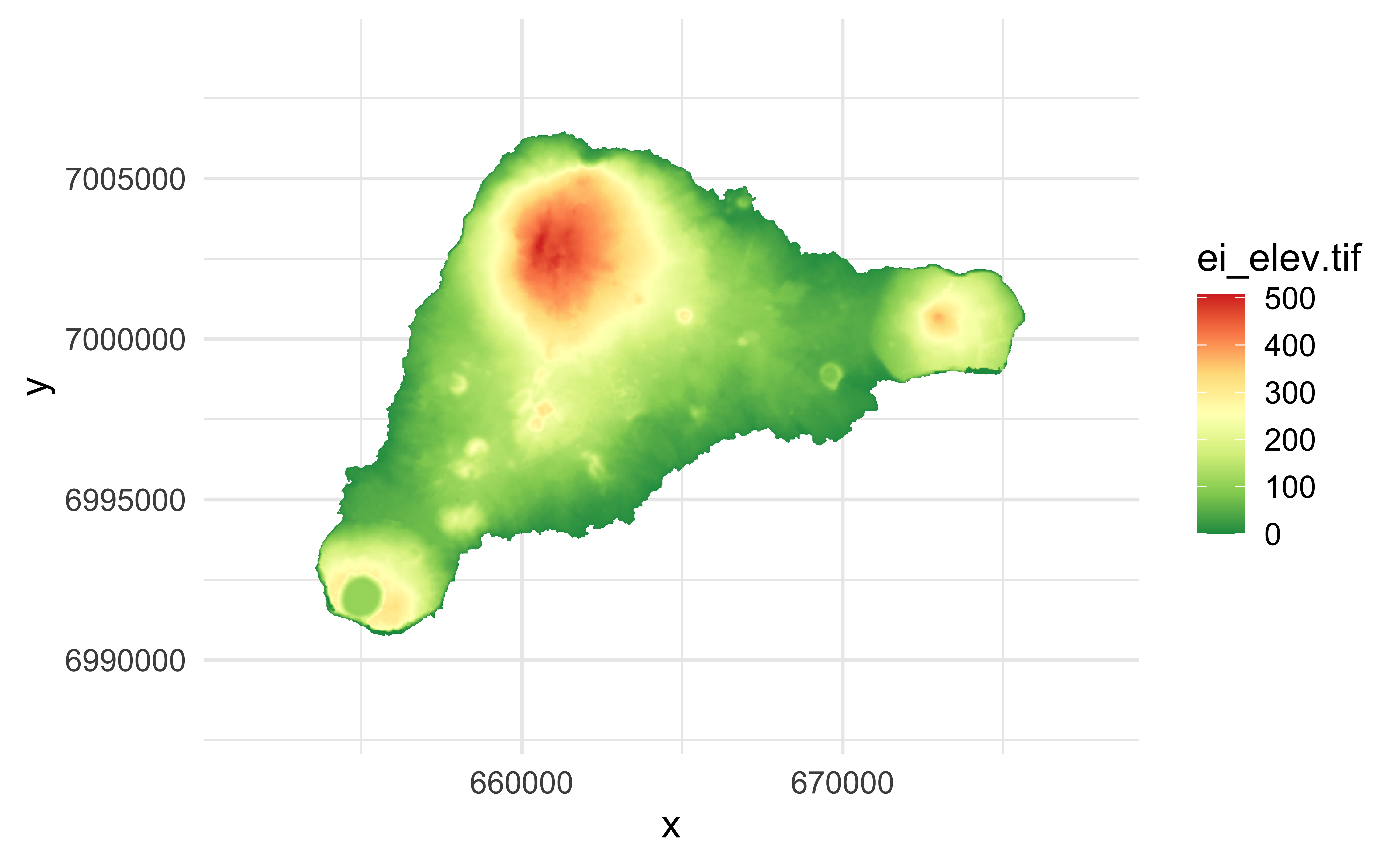
File types

  • tif files are geospatial raster data, e.g., elevation maps

  • gpkg are geopackage files, modern version of shapefiles

Reading tif files

elev <- read_stars("data/easter_island/ei_elev.tif")
elev
stars object with 2 dimensions and 1 attribute
attribute(s):
             Min.  1st Qu.   Median     Mean  3rd Qu.     Max.
ei_elev.tif     0 56.98041 114.3601 143.5146 204.9752 506.8161
               NA's
ei_elev.tif  619721
dimension(s):
  from   to  offset delta                refsys point x/y
x    1 1060  651409    25 WGS 84 / UTM zone 12S FALSE [x]
y    1  832 7008921   -25 WGS 84 / UTM zone 12S FALSE [y]

Plotting tif files

ggplot() +
  geom_stars(data = elev)

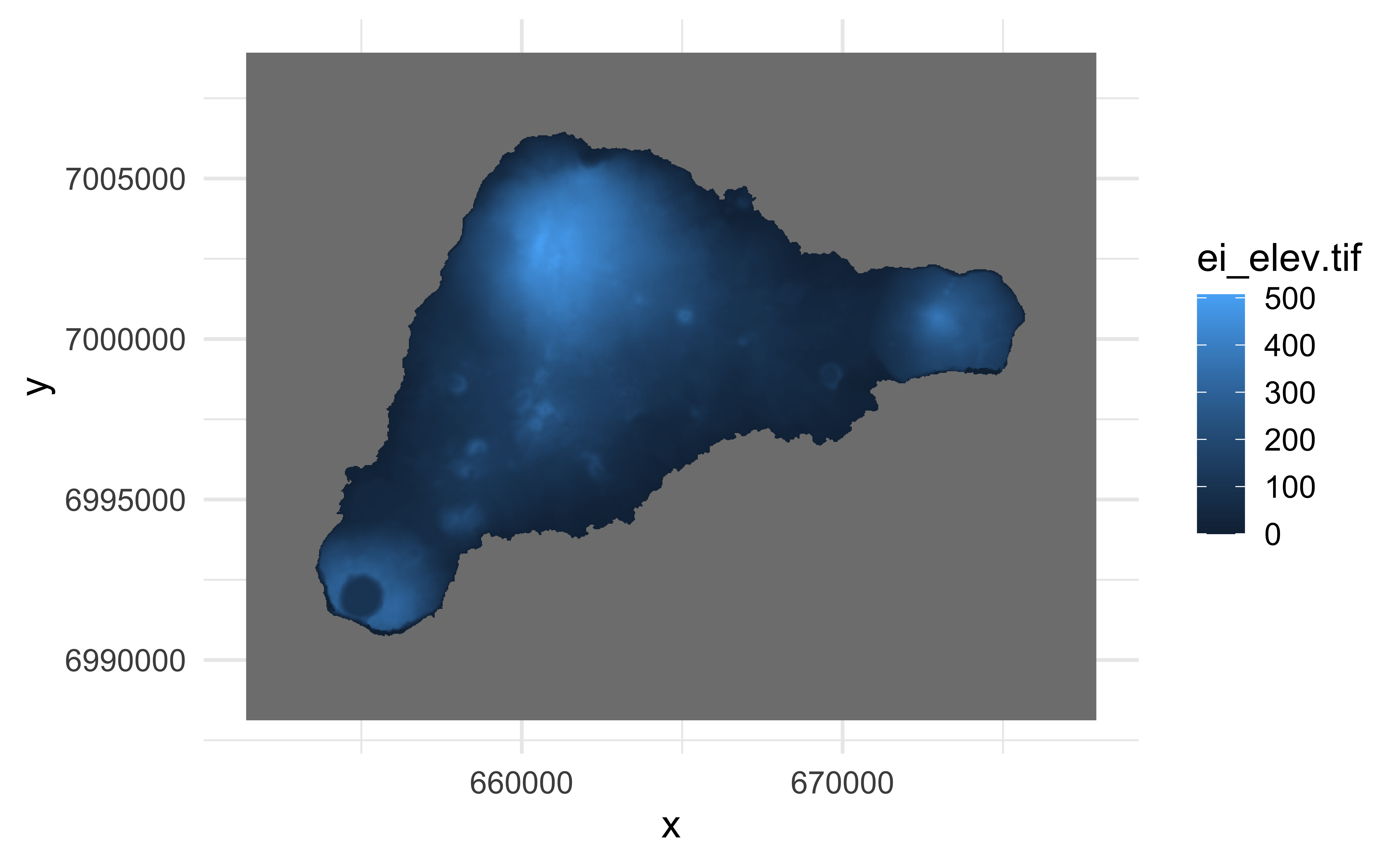
Plays nicely with ggplot2
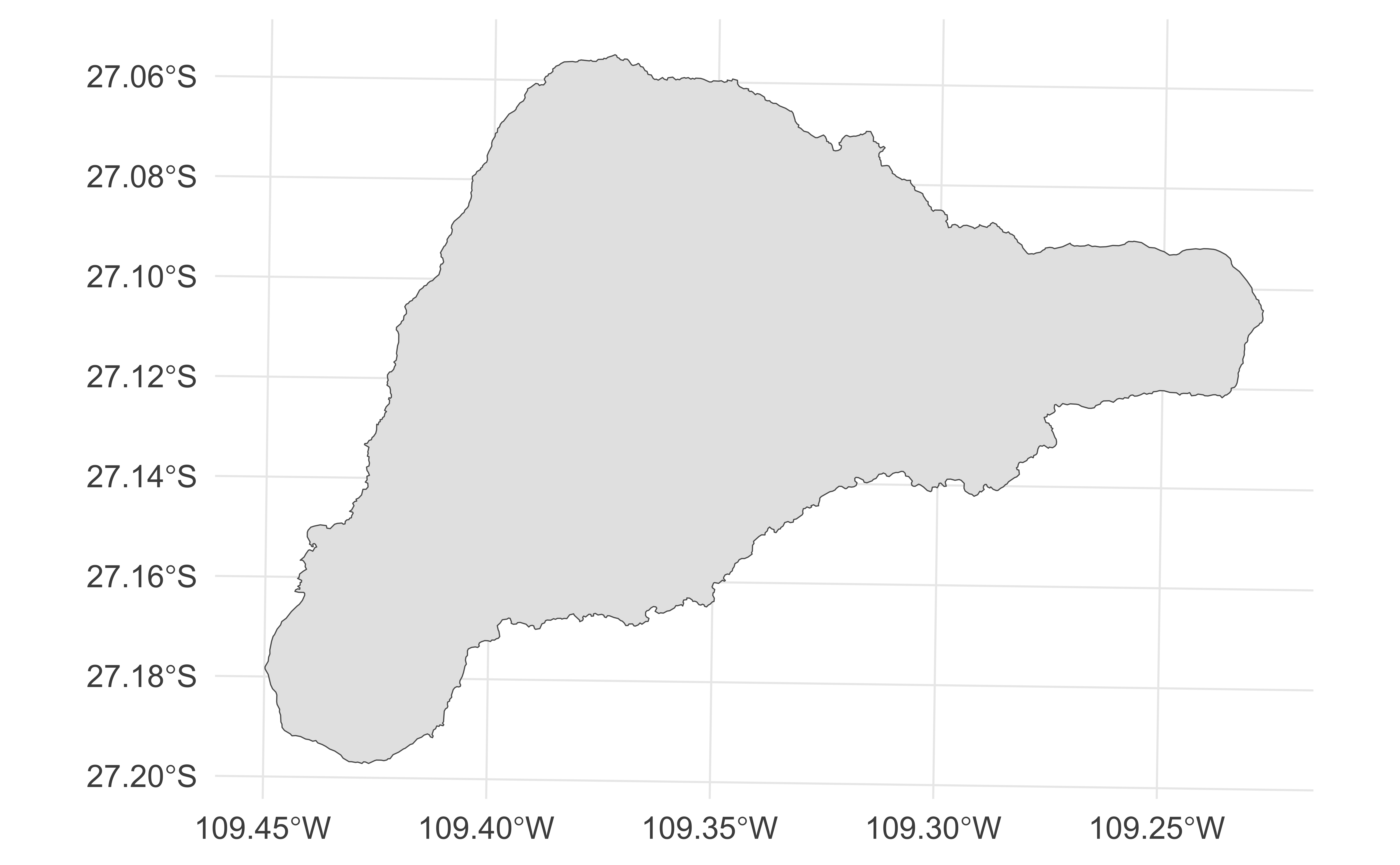
ggplot() +
  geom_stars(data = elev) +
  scale_fill_distiller(palette = "RdYlGn", na.value = "transparent")

Reading gpkg files

border <- read_sf("data/easter_island/ei_border.gpkg")
border
Simple feature collection with 1 feature and 1 field
Geometry type: POLYGON
Dimension:     XY
Bounding box:  xmin: 653566.4 ymin: 6990751 xmax: 675697.4 ymax: 7006462
Projected CRS: WGS 84 / UTM zone 12S
# A tibble: 1 × 2
  name                                                       geom
  <chr>                                             <POLYGON [m]>
1 Rapa Nui / Isla de Pascua ((668715.4 7002628, 668776.6 7002640…

Plotting gpkg files

ggplot() +
  geom_sf(data = border)

A brief aside…

Put a flag on it!

Just for fun…

ei_plot <- ggplot() +
  geom_sf(data = border, fill = "white")

ei_flag_image <- image_read("images/Flag_of_Rapa_Nui_Chile.png")
ei_flag_raster <- as.raster(ei_flag_image)

ei_plot + annotation_raster(ei_flag_raster, xmin = 657000, xmax = 670000, ymin = 6996000, ymax = 7004000)

Put a flag on it!

Finding the “bounding box”

  • ggplot_build() takes the plot object, and performs all steps necessary to produce an object that can be rendered
  • Outputs:
    1. a list of data frames (one for each layer)
    2. a panel object, which contain all information about axis limits, breaks etc.
ei_plot_build <- ggplot_build(ei_plot)

ggplot_build()

ei_plot_build
$data
$data[[1]]
                        geometry PANEL group     xmin     xmax
1 POLYGON ((668715.4 7002628,...     1    -1 653566.4 675697.4
     ymin    ymax linetype alpha stroke  fill
1 6990751 7006462        1    NA    0.5 white


$layout
<ggproto object: Class Layout, gg>
    coord: <ggproto object: Class CoordSf, CoordCartesian, Coord, gg>
        aspect: function
        backtransform_range: function
        clip: on
        crs: NULL
        datum: crs
        default: TRUE
        default_crs: NULL
        determine_crs: function
        distance: function
        expand: TRUE
        fixup_graticule_labels: function
        get_default_crs: function
        is_free: function
        is_linear: function
        label_axes: list
        label_graticule: 
        labels: function
        limits: list
        lims_method: cross
        modify_scales: function
        ndiscr: 100
        params: list
        range: function
        record_bbox: function
        render_axis_h: function
        render_axis_v: function
        render_bg: function
        render_fg: function
        setup_data: function
        setup_layout: function
        setup_panel_guides: function
        setup_panel_params: function
        setup_params: function
        train_panel_guides: function
        transform: function
        super:  <ggproto object: Class CoordSf, CoordCartesian, Coord, gg>
    coord_params: list
    facet: <ggproto object: Class FacetNull, Facet, gg>
        compute_layout: function
        draw_back: function
        draw_front: function
        draw_labels: function
        draw_panels: function
        finish_data: function
        init_scales: function
        map_data: function
        params: list
        setup_data: function
        setup_params: function
        shrink: TRUE
        train_scales: function
        vars: function
        super:  <ggproto object: Class FacetNull, Facet, gg>
    facet_params: list
    finish_data: function
    get_scales: function
    layout: data.frame
    map_position: function
    panel_params: list
    panel_scales_x: list
    panel_scales_y: list
    render: function
    render_labels: function
    reset_scales: function
    setup: function
    setup_panel_guides: function
    setup_panel_params: function
    train_position: function
    xlabel: function
    ylabel: function
    super:  <ggproto object: Class Layout, gg>

$plot

attr(,"class")
[1] "ggplot_built"

Diving into the output

ei_plot_build$data[[1]]$xmin
[1] 653566.4
ei_plot_build$data[[1]]$xmax
[1] 675697.4
ei_plot_build$data[[1]]$ymin
[1] 6990751
ei_plot_build$data[[1]]$ymax
[1] 7006462

Back to Easter Island…

Let’s get more data

roads <- read_sf("data/easter_island/ei_roads.gpkg")
points <- read_sf("data/easter_island/ei_points.gpkg")

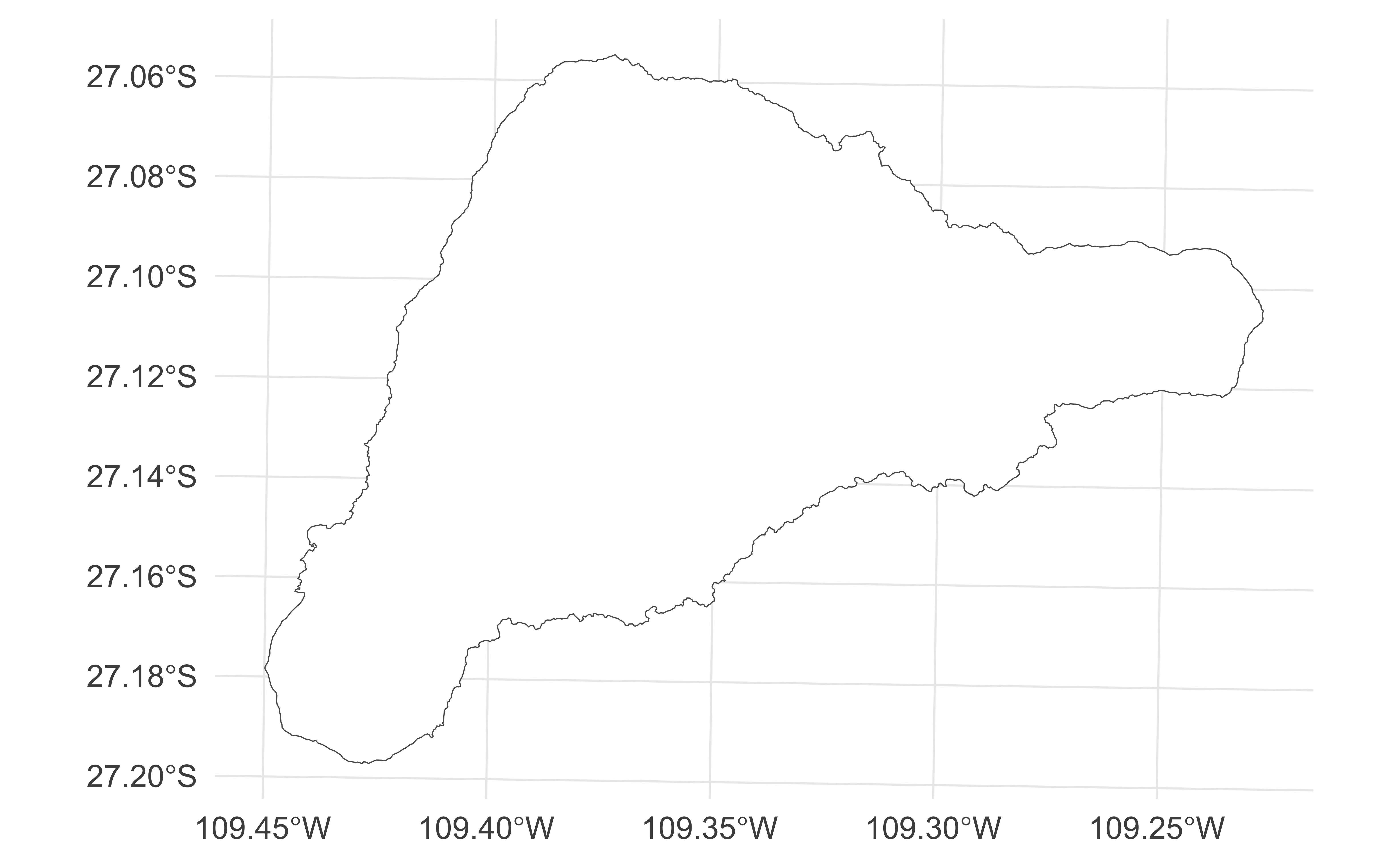
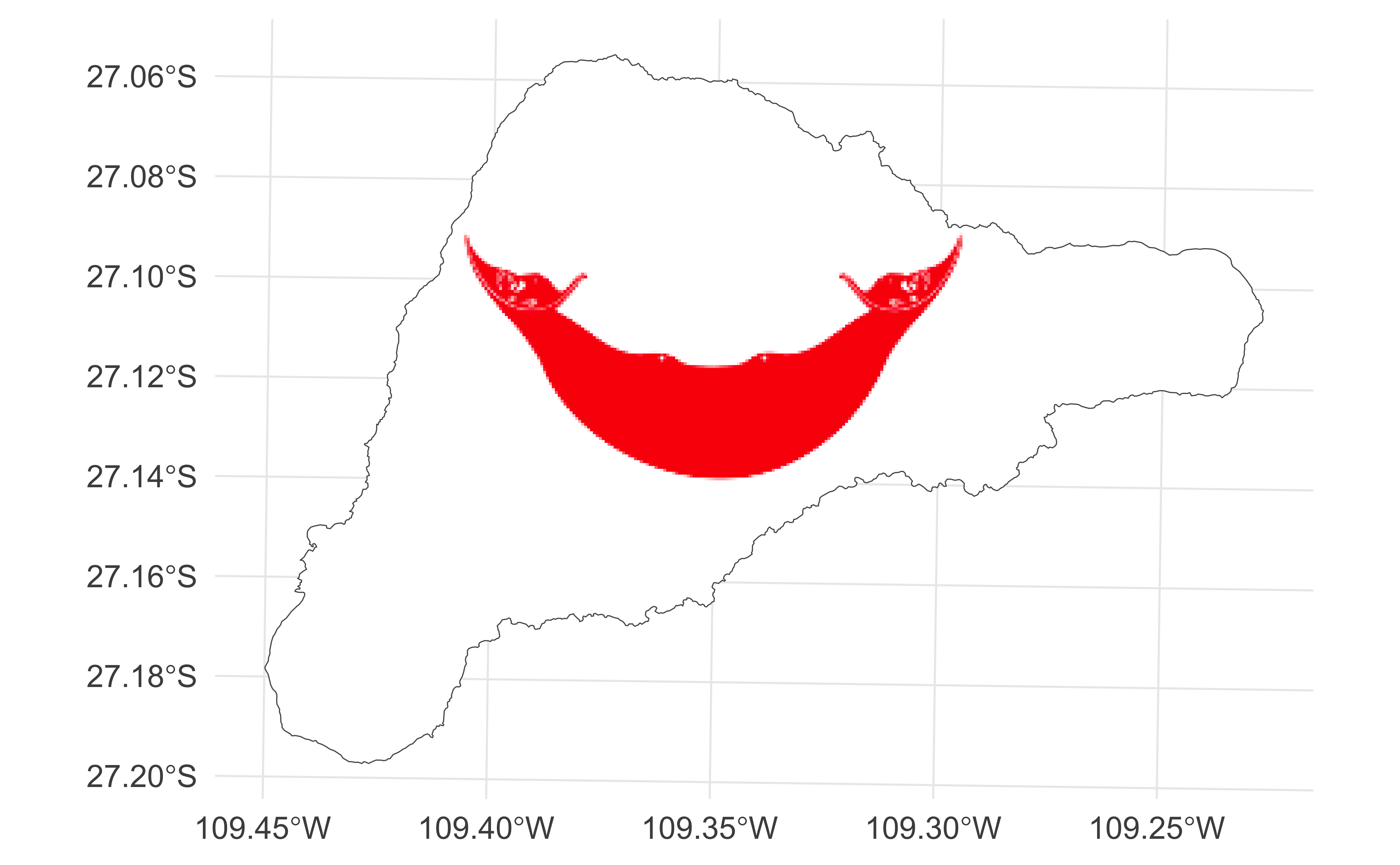
Layering with ggplot2

ae-18: Recreate the visualization below.