# load packages
library(countdown)
library(tidyverse)
library(ggrepel)
library(ggspatial)
library(patchwork)
library(rnaturalearth)
library(rnaturalearthdata)
library(sf)

# set theme for ggplot2
ggplot2::theme_set(ggplot2::theme_minimal(base_size = 14))

# set width of code output
options(width = 65)

# set figure parameters for knitr
knitr::opts_chunk$set(
  fig.width = 7, # 7" width
  fig.asp = 0.618, # the golden ratio
  fig.retina = 3, # dpi multiplier for displaying HTML output on retina
  fig.align = "center", # center align figures
  dpi = 300 # higher dpi, sharper image
)Visualizing geospatial data II
Lecture 19
The sf package
A package that provides simple features access for R:
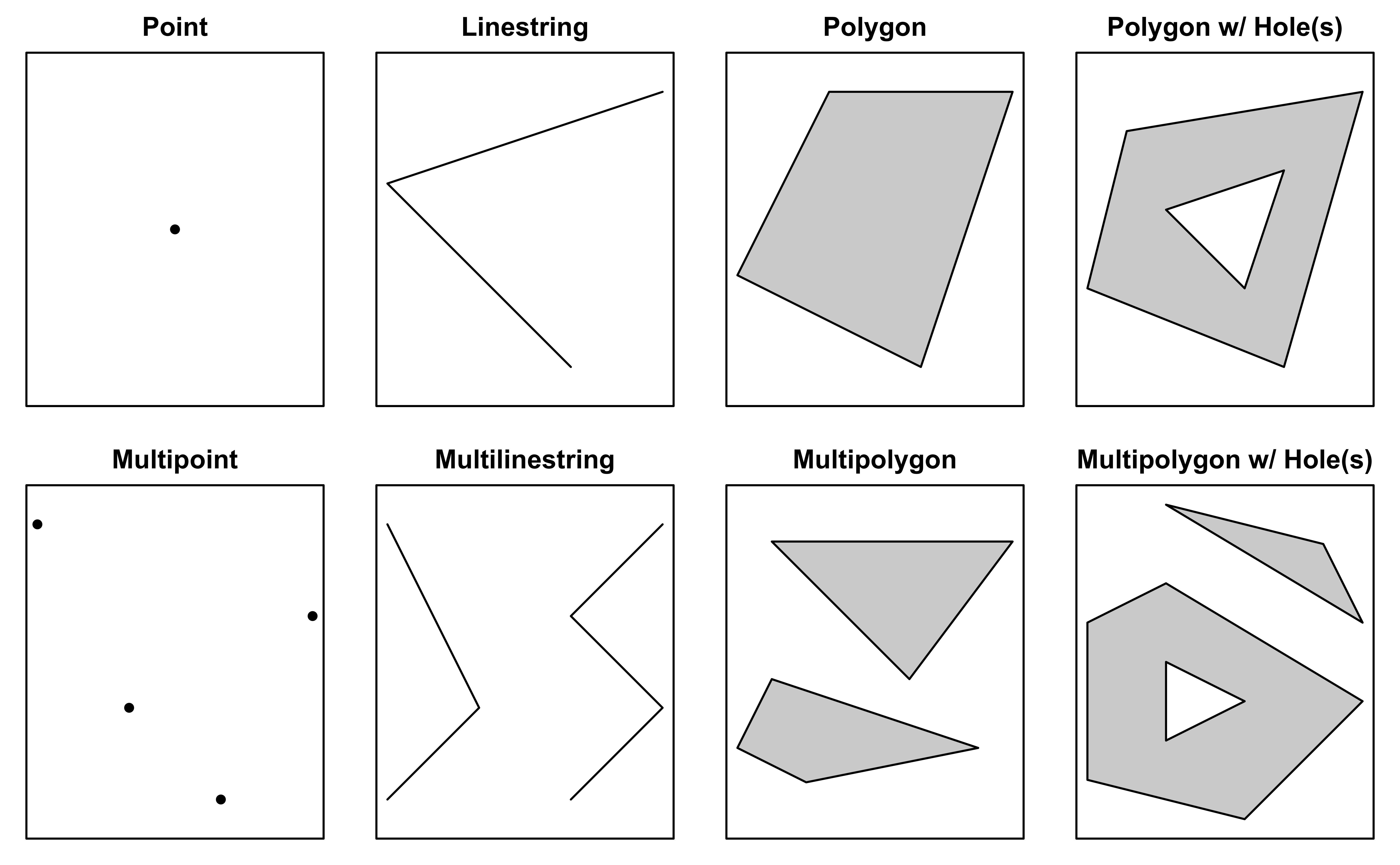
- represents simple features as records in a
data.frameortibblewith ageometrylist-column - represents natively in R all 17 simple feature types for all dimensions
Learn more at r-spatial.github.io/sf.

Simple Features for R
Simple Features
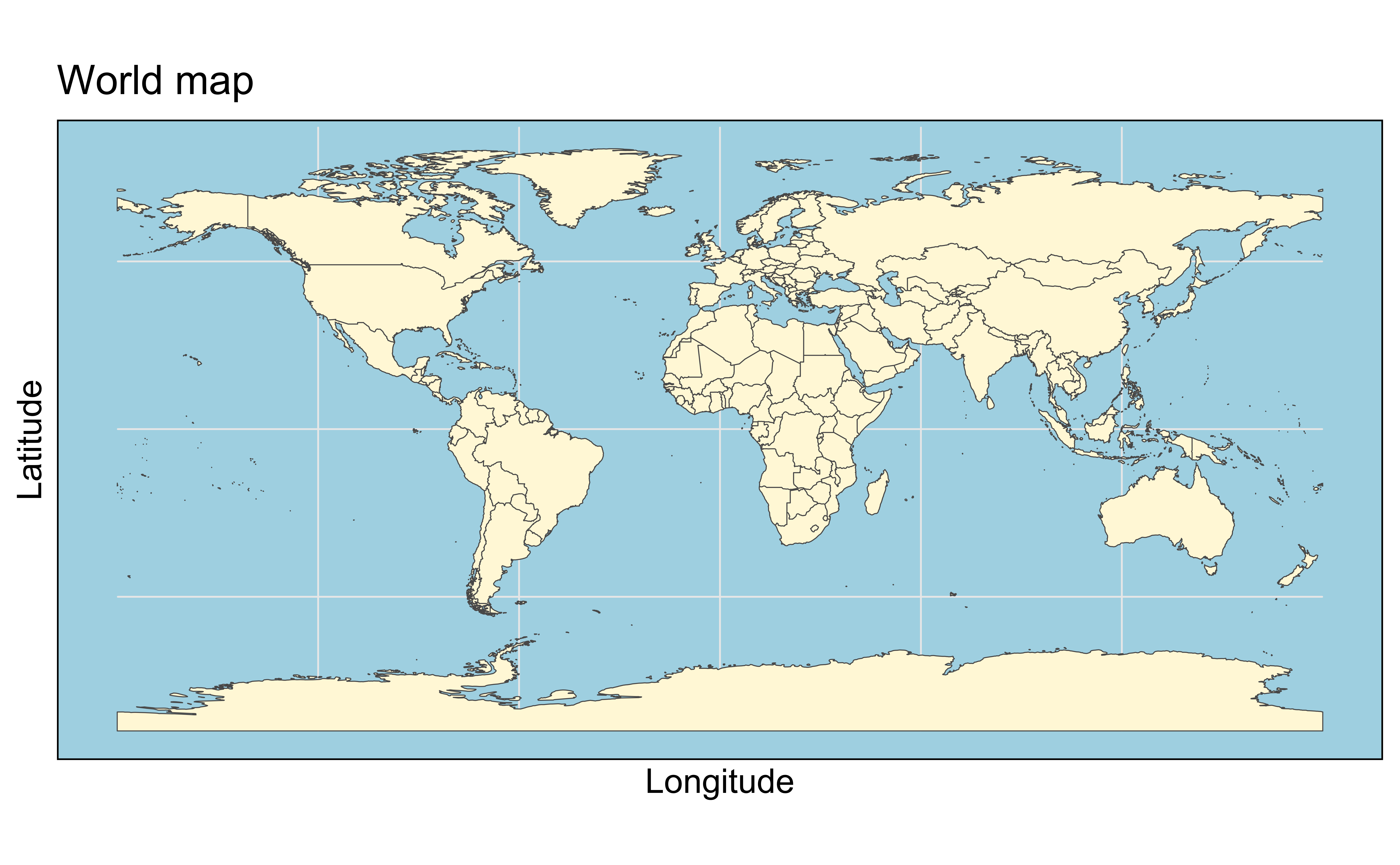
Map the world with sf

Plays nicely with ggplot2
Plays nicely with ggplot2

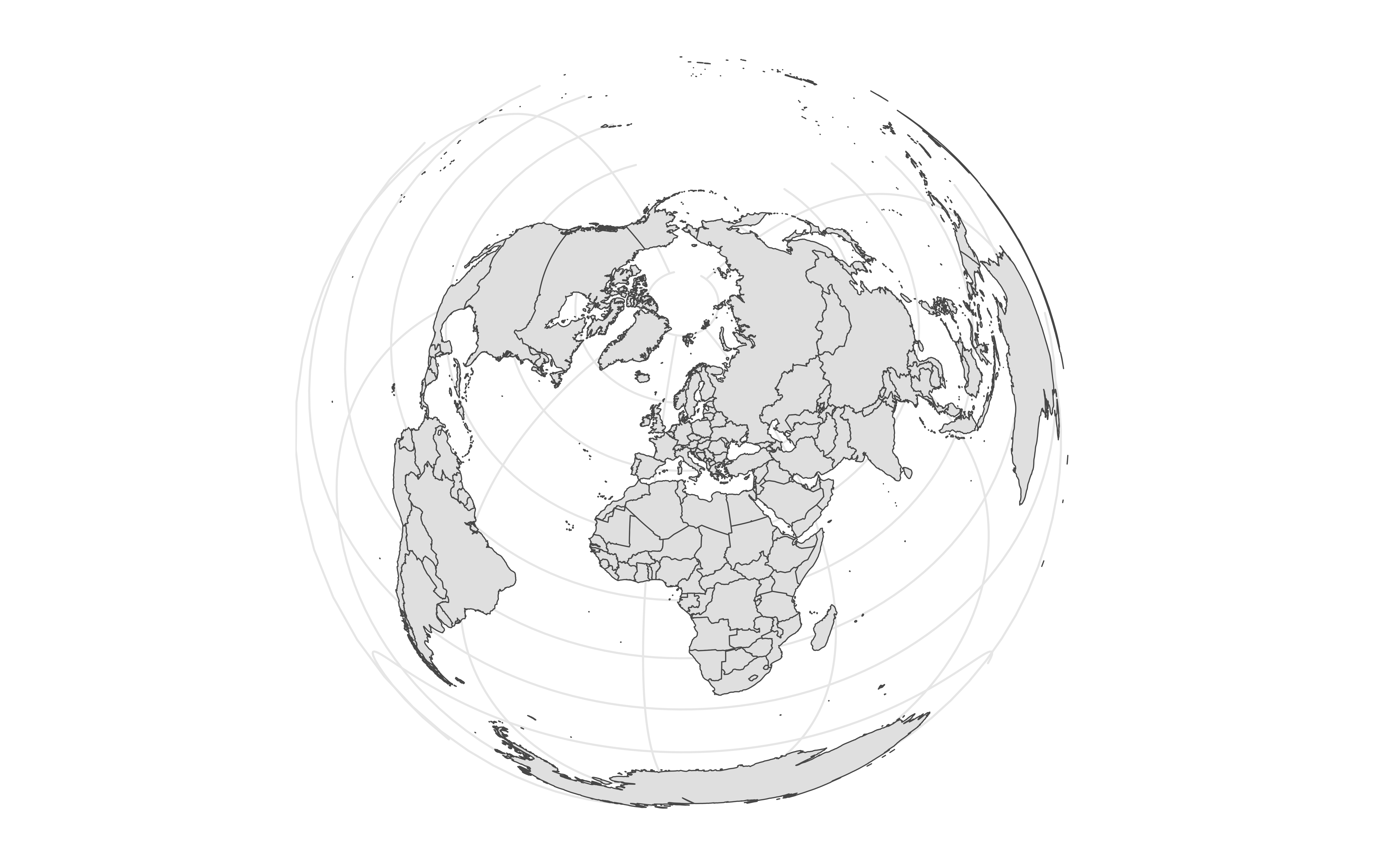
Projections with sf
Scale bar and North arrow
Scale on map varies by more than 10%, scale bar may be inaccurate
Projections
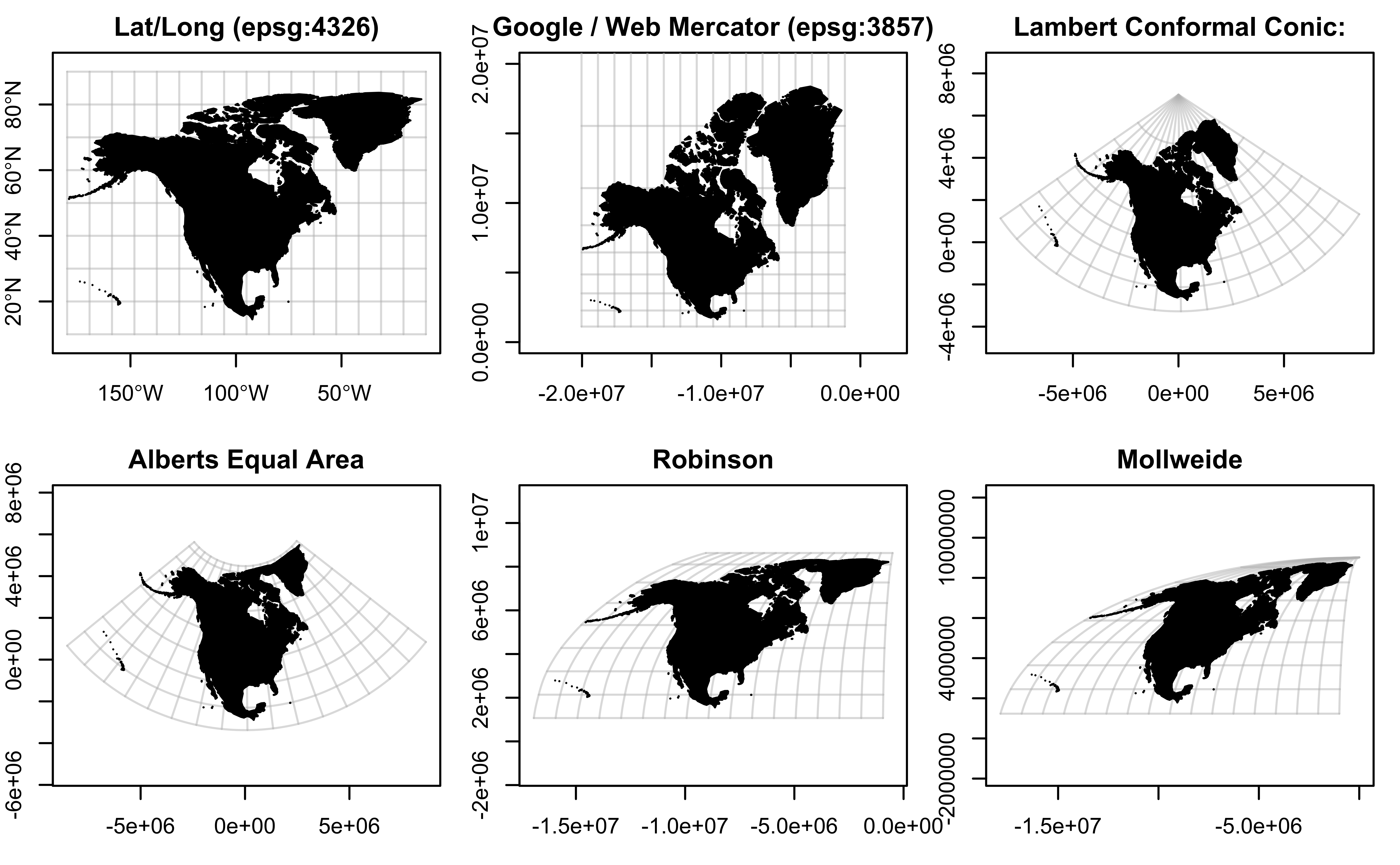
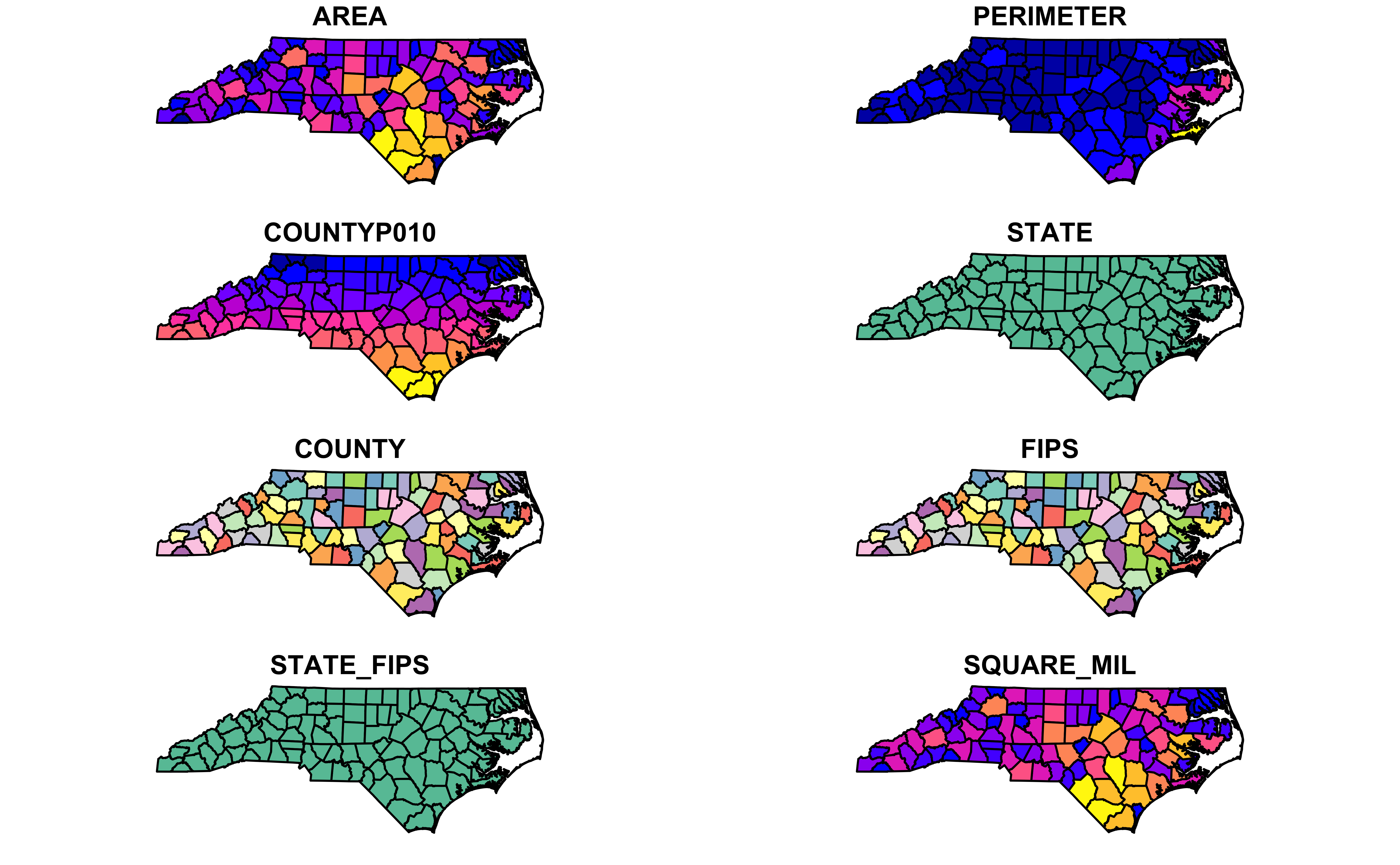
All variables at once
Where did these variables come from? Which of these plots don’t make sense?
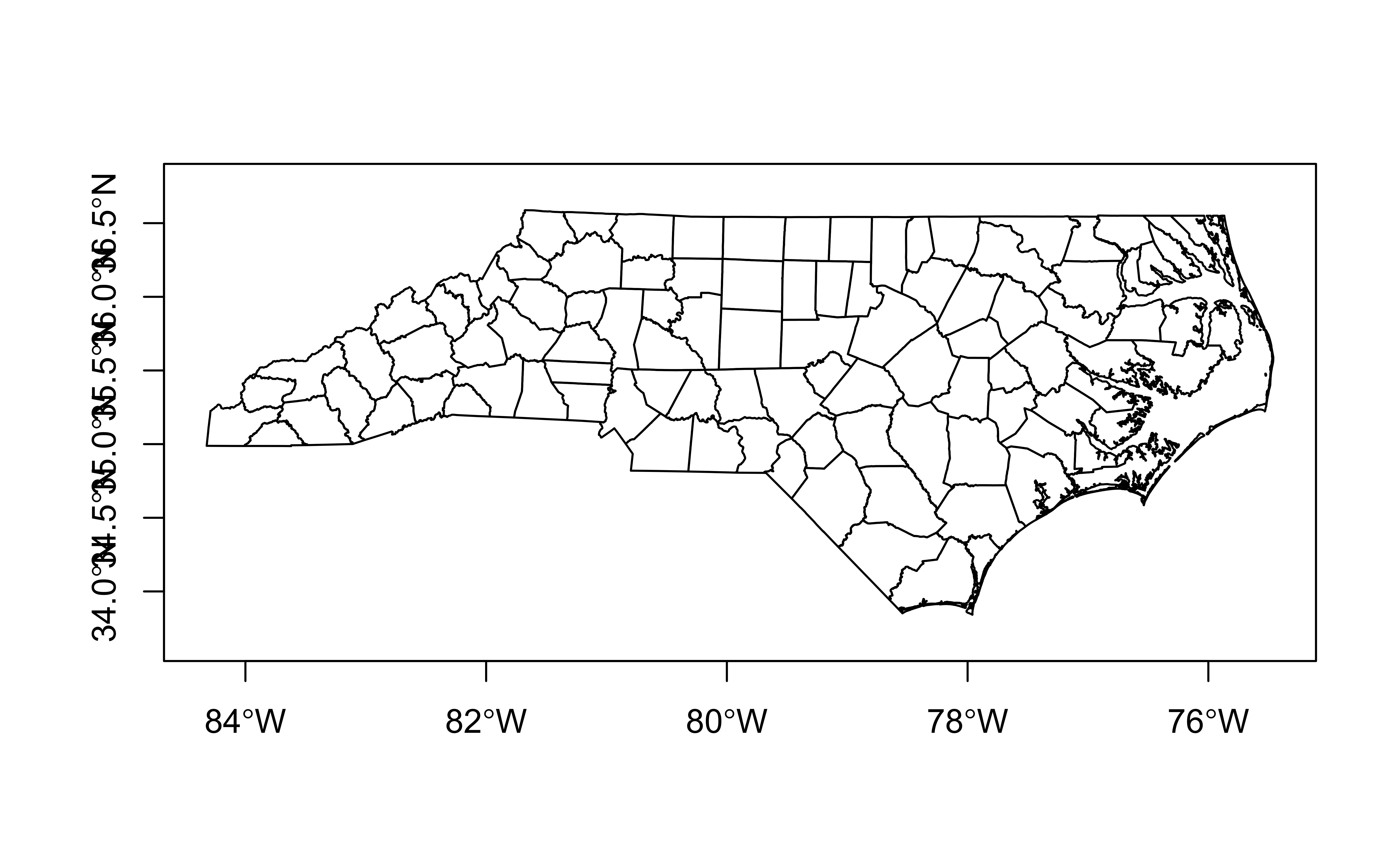
Geometry Plot
Graticules
Graticules

Graticules (EPSG:3631)

Graticules (EPSG:3631)
Graticules (EPSG:3631)

geom_sf()
No automatic plotting:
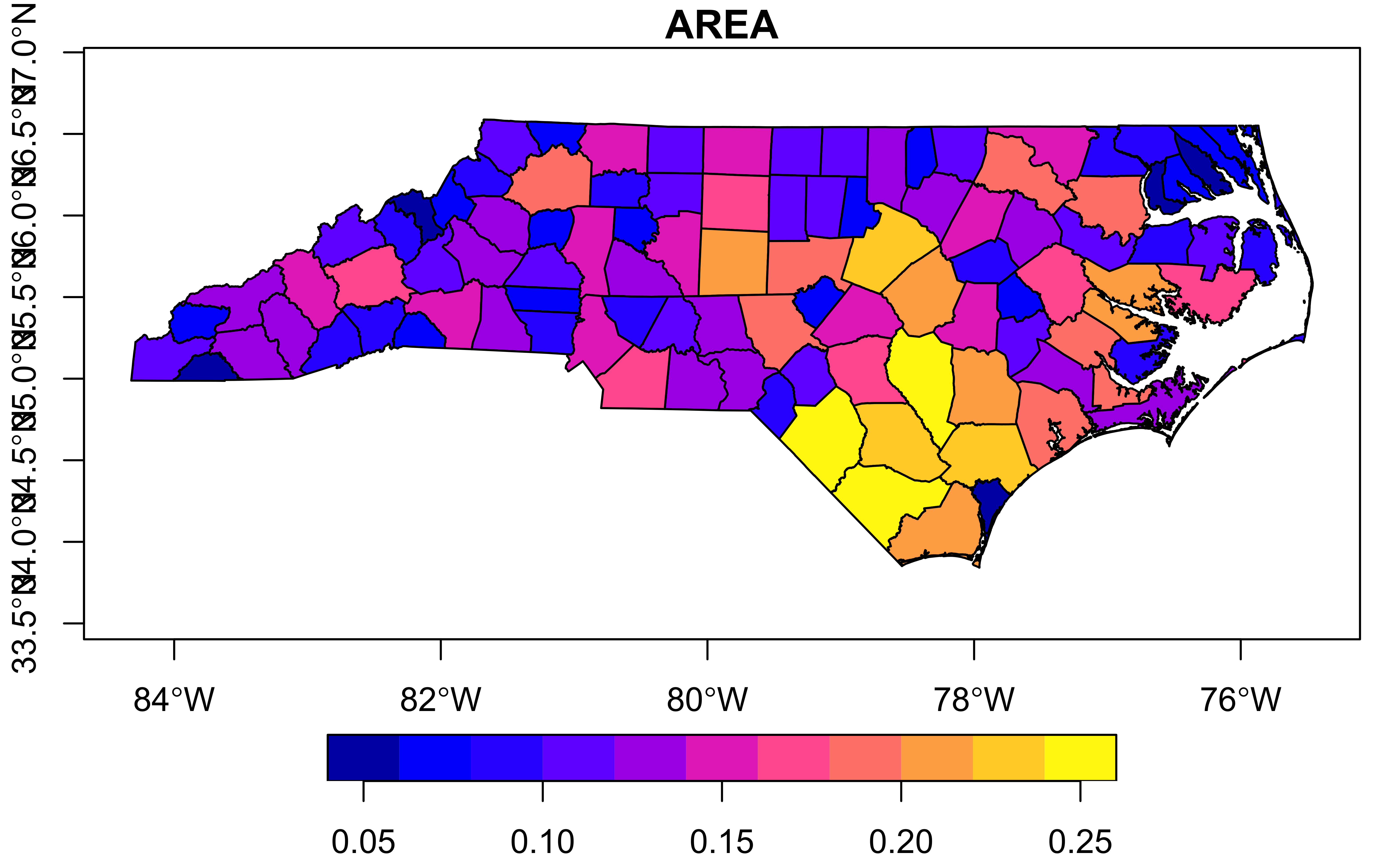
aes()thetic mappings
More expressive: to plot variables, use aesthetic mappings as usual:
Many variables at once
Using patchwork:
ggplot2 + projections
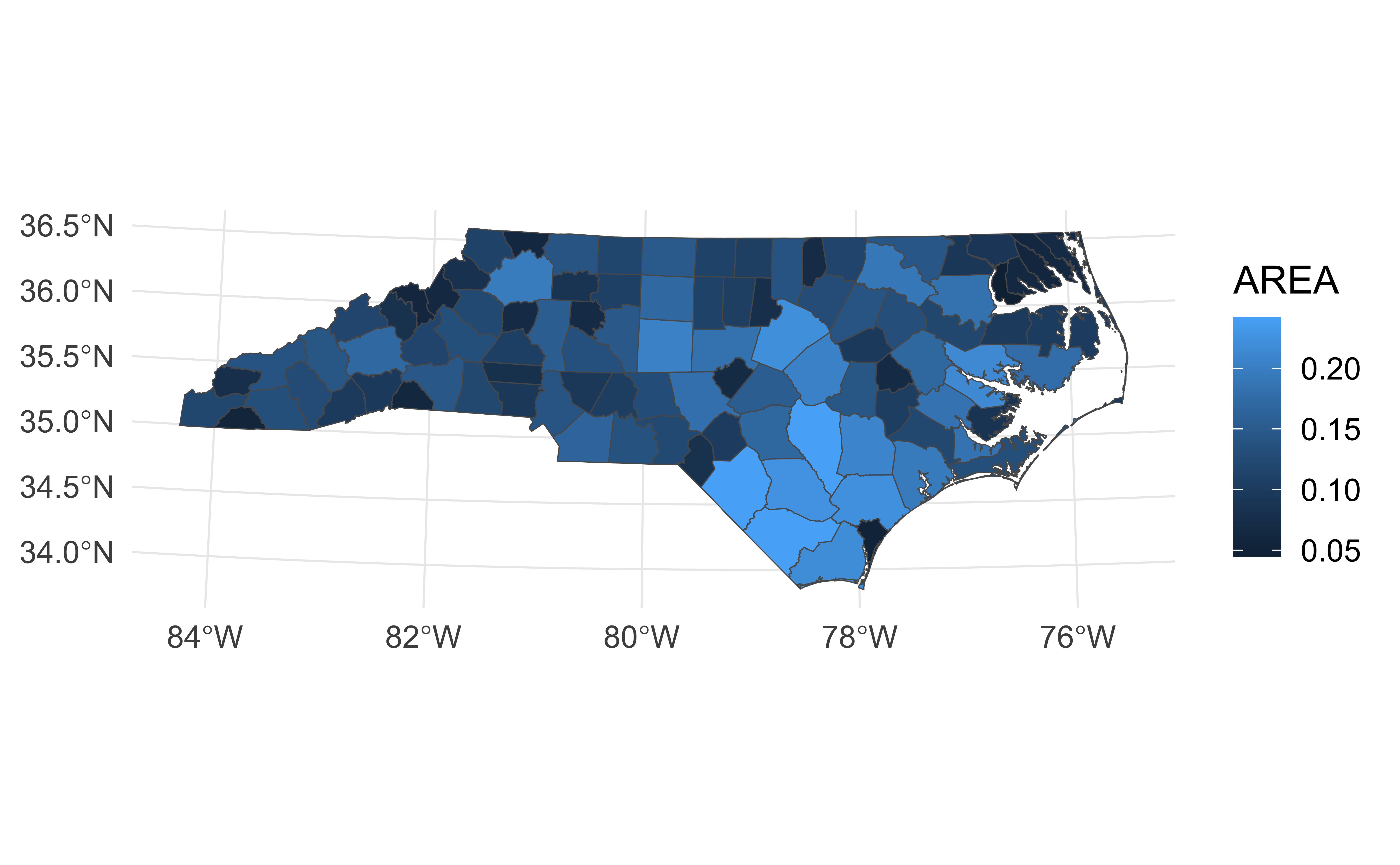
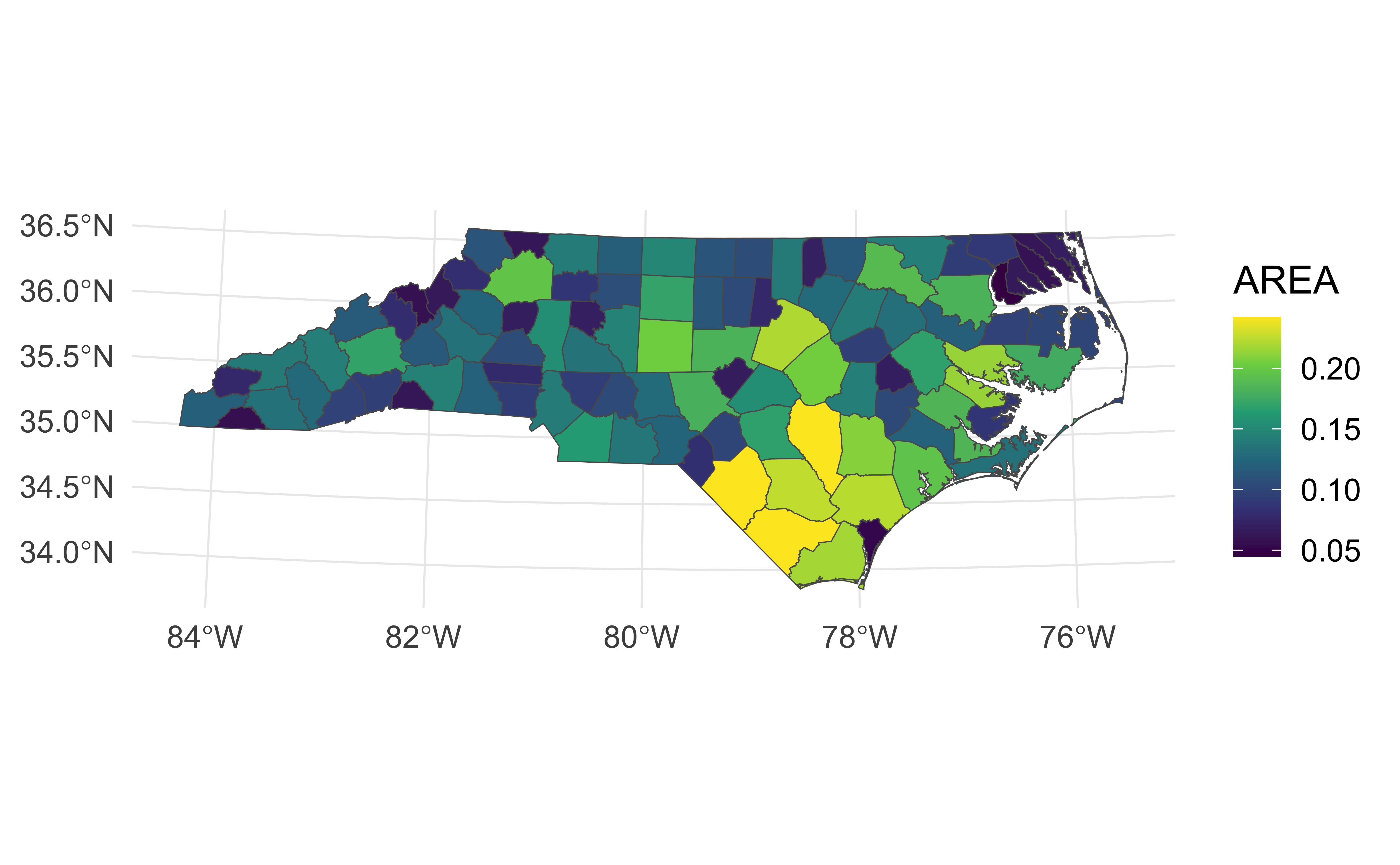
ggplot2 + viridis
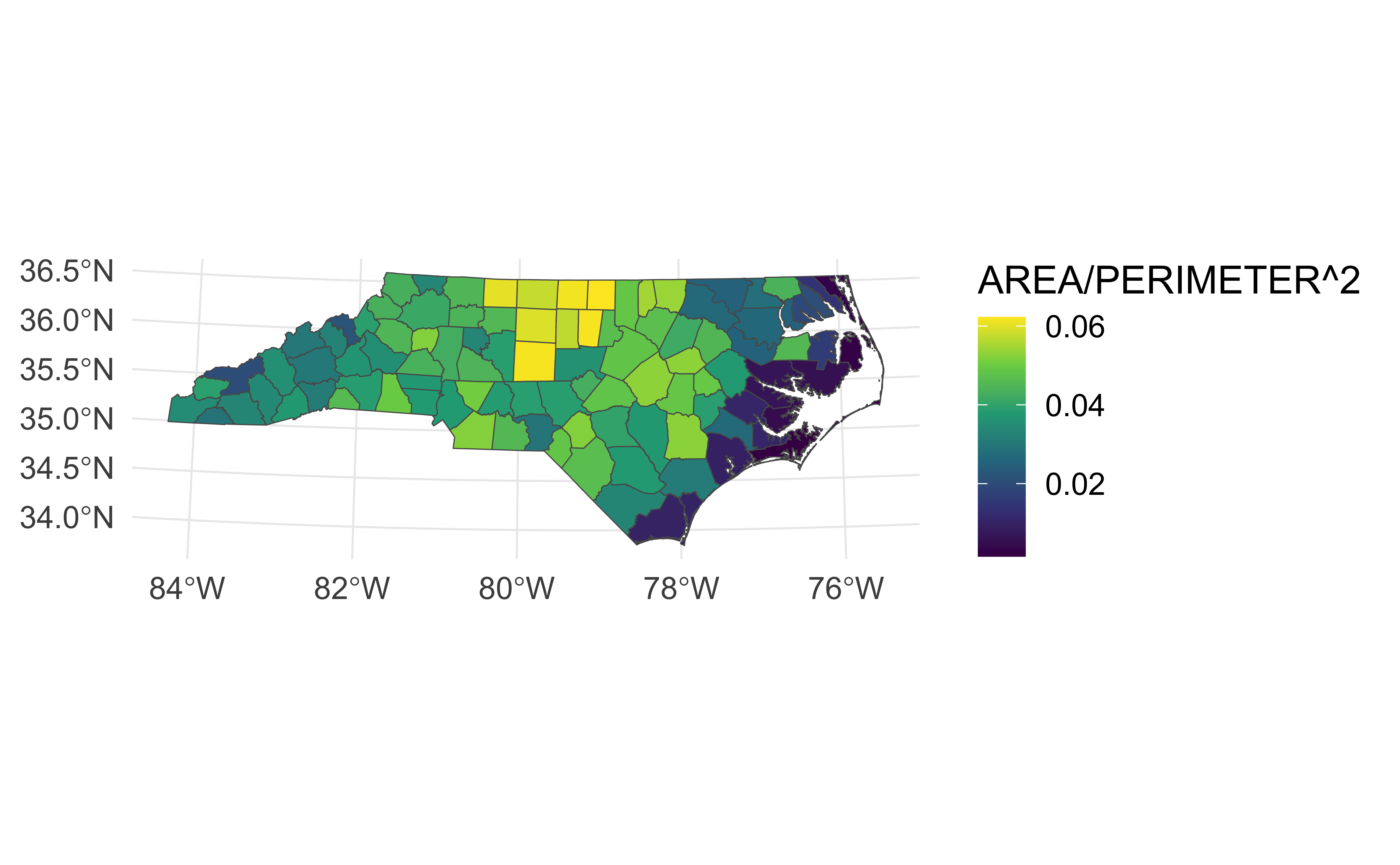
ggplot2 + calculations
Other color palettes (discrete)
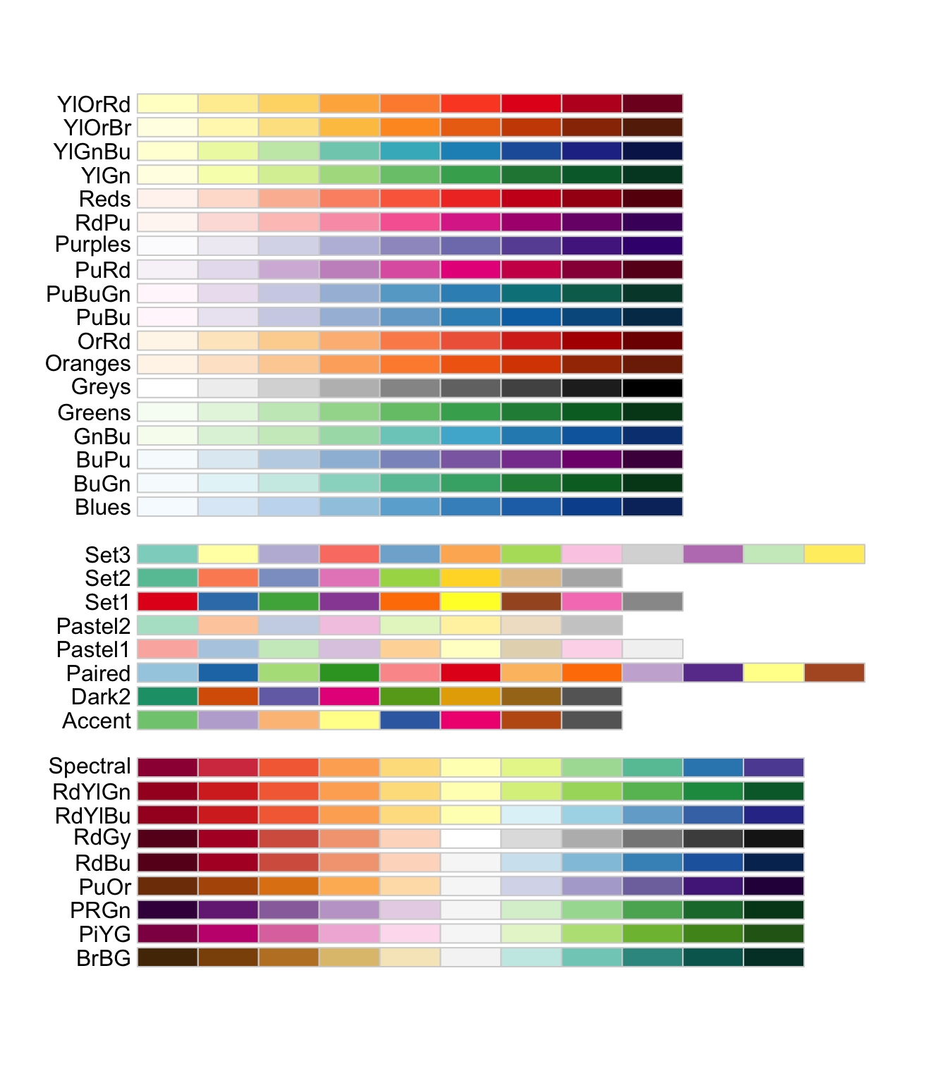
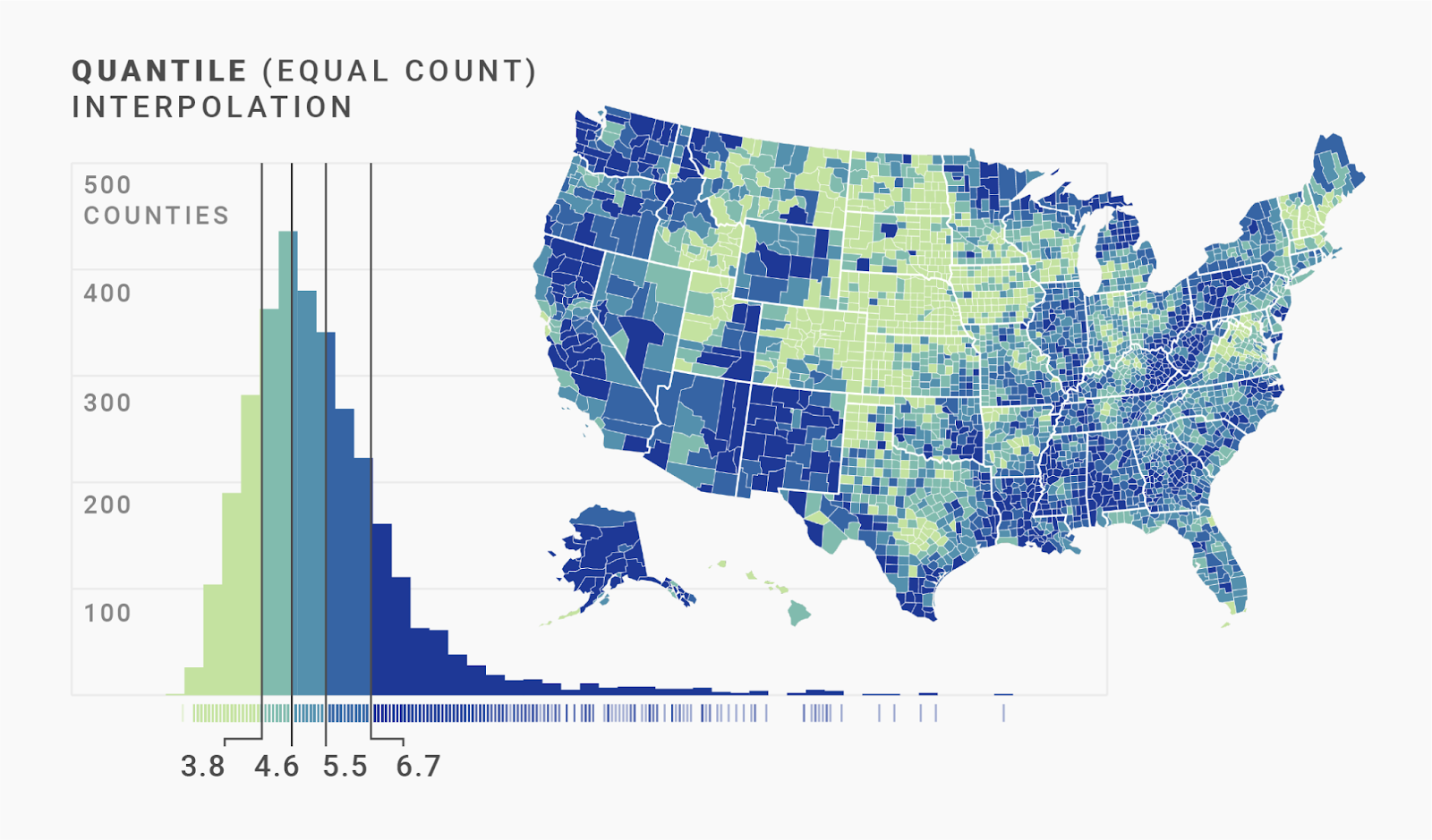
Picking palette breaks
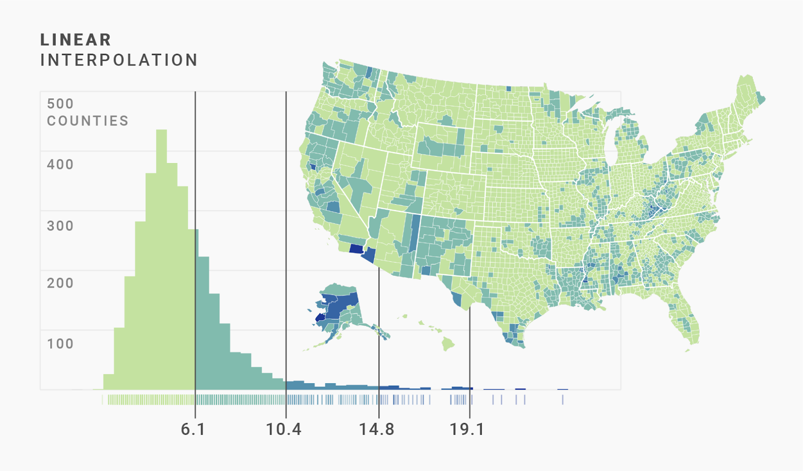
Picking palette breaks
Data
ggplot(data = nc) +
geom_sf() +
labs(title = "NC Counties")
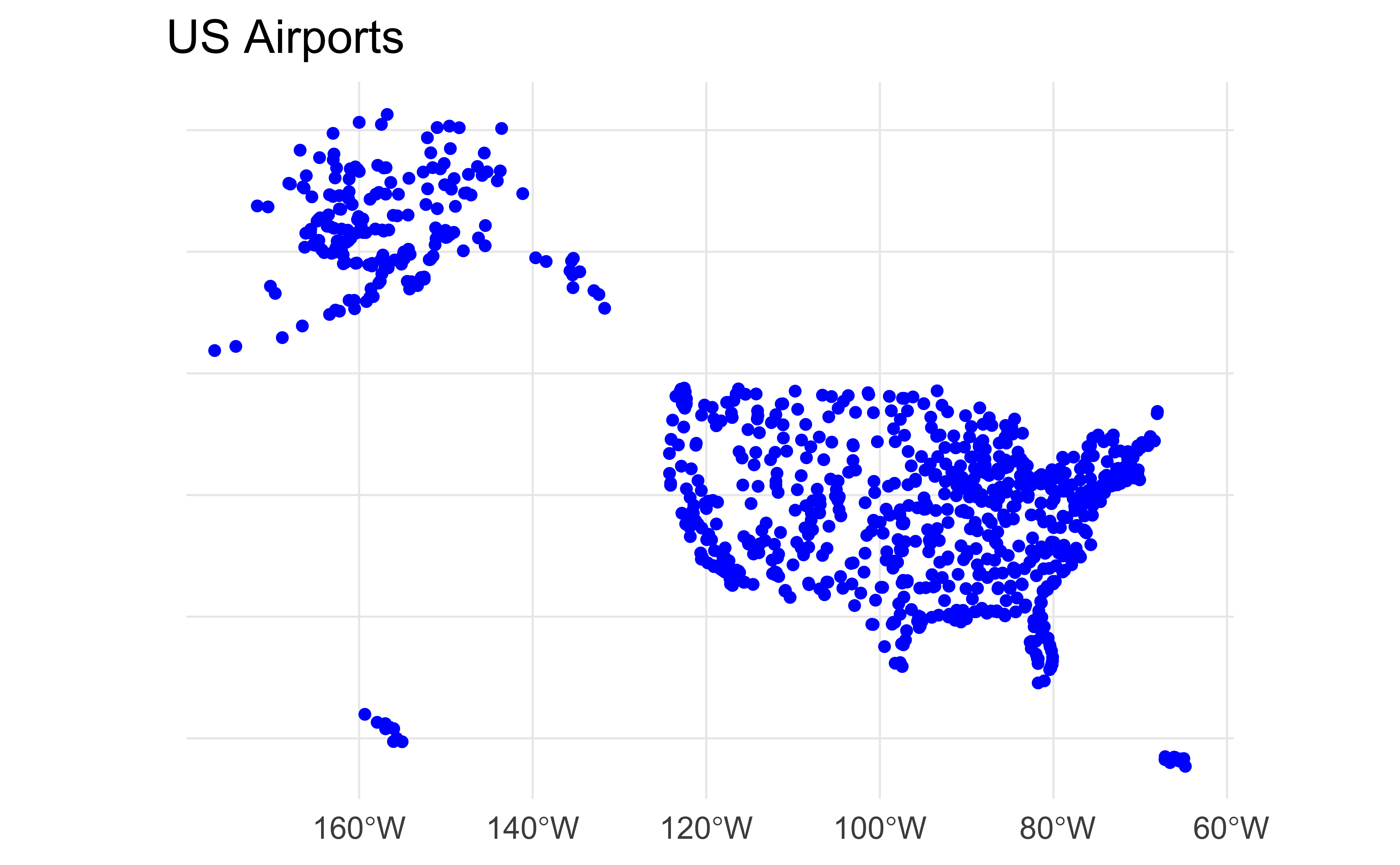
ggplot(data = air) +
geom_sf(color = "blue") +
labs(title = "US Airports")
ggplot(data = hwy) +
geom_sf(color = "orange") +
labs(title = "US Highways")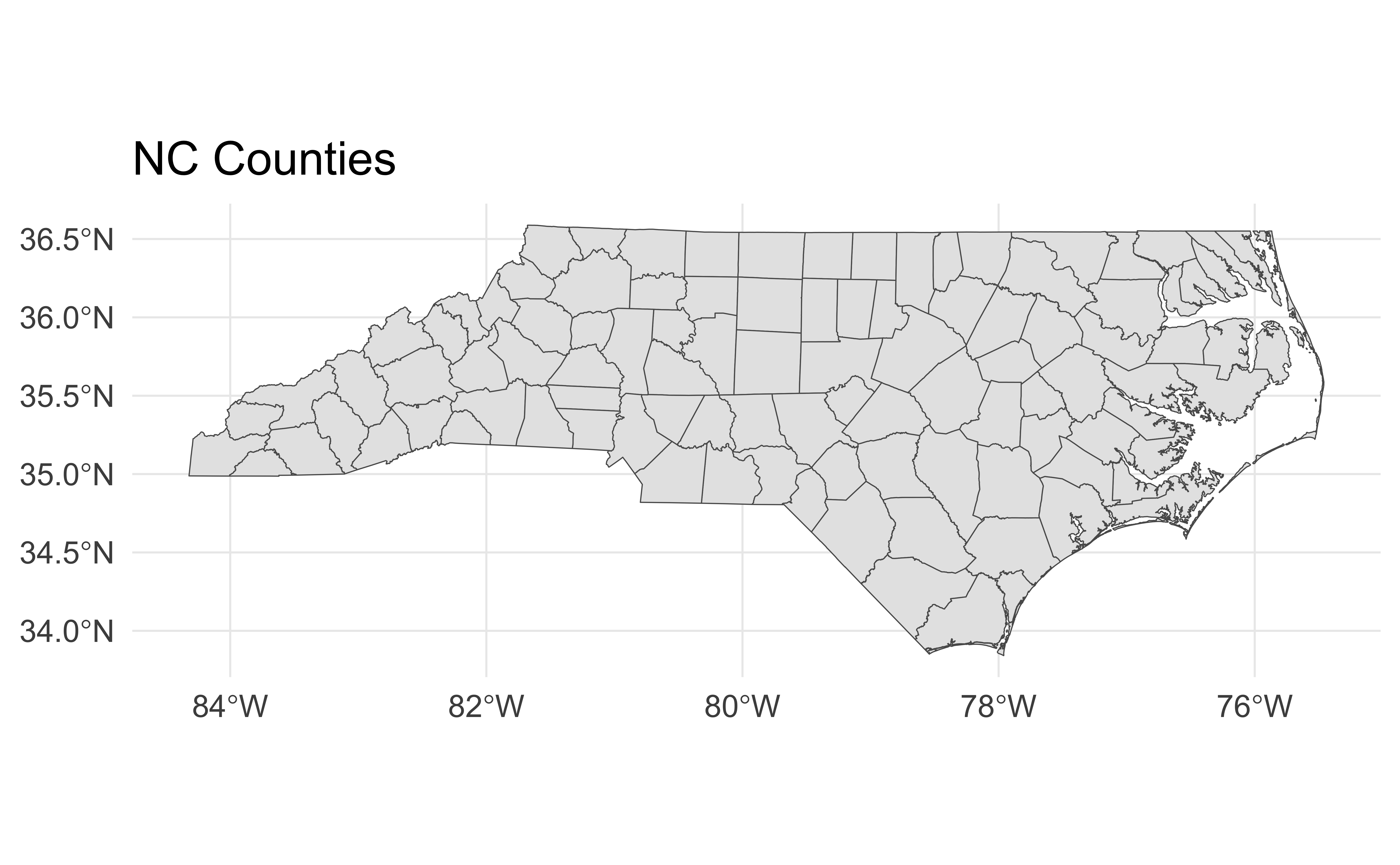
Layering
ae-17: Recreate the following visualization.
Which counties have airports?
ae-17: On the map of NC you made previously, highlight the counties that have airports.
![]()